Given a collection of data that may fit the PERT distribution, we would like to estimate the parameters which best fit the data. We illustrate the method of moments approach on this webpage. Click here to see another approach, using the maximum likelihood method.
Using Equations
Given a data set X with elements x1, …, xn, our objective is to estimate the parameters of a PERT distribution that best fits the data set.
The PERT distribution has three parameters a < b < c. Clearly
a ≤ min X max X ≤ c
Estimating b from a and c
If you know the values of a (the left end-point) and c (the right end-point) parameters, then you can use these values to estimate b (the mode) based on the formula for the mean m, namely
Hence
Estimating a and b from c
If you know the value of c, then you can estimate a and b based on the sample mean m and standard deviation s, as follows:
Hence
Similarly, if we know the value of a then
Estimating all three parameters
If we don’t know the value of any of the parameters, we can use the skewness of the data in X
where
Property 1: If the data set X follows a PERT distribution, we can use the above formulas for the PERT distribution setting them equal to the sample mean m, standard deviation s, and skewness w values to obtain estimates for the a, b, and c parameters. In particular
Here the sign + or – is the one that produces the best estimate of skewness.
Proof: Click here for the details.
The parameters a and b can then be estimated from a = c – 6s and b = (3m + 3s – c).
Example
Example 1: Fit the data in range B2:G11 of Figure 1 to a PERT distribution using the method of moments.
Using Property 1, we obtain the values for a, b, and c shown in the range M2:M4. We can see that the mean, variance, and skewness for the PERT distribution based on these parameters are almost identical to sample statistics. In particular, the sum of squares shown in cell M12 is close to zero.
Figure 1 – Method of Moments
The only problem is that a = 1.34507 > 1.134794 = min X, which is impossible. This is also reflected in the error value for LL based on these parameters, as shown in cell M14.
Using Solver
Example 2: Use Excel’s Solver to fit the data in range B2:G11 of Figure 1 to a PERT distribution using the method of moments.
Figure 2 – Fitting a PERT distribution using Solver
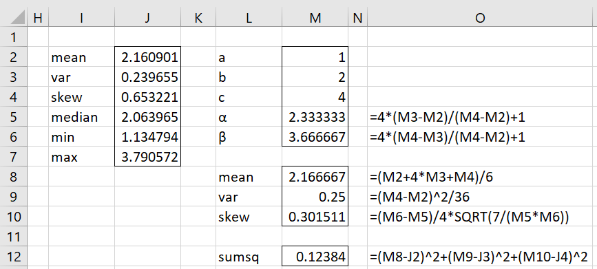
To accomplish this, set a, b, and c to some initial values as shown in Figure 2, and then select Data > Analyze|Solver, and fill in the dialog box shown in Figure 3.
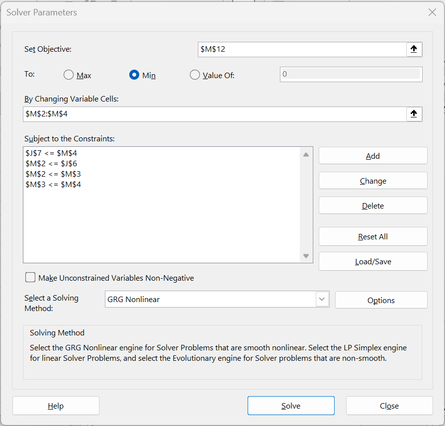
Figure 3 – Solver dialog box
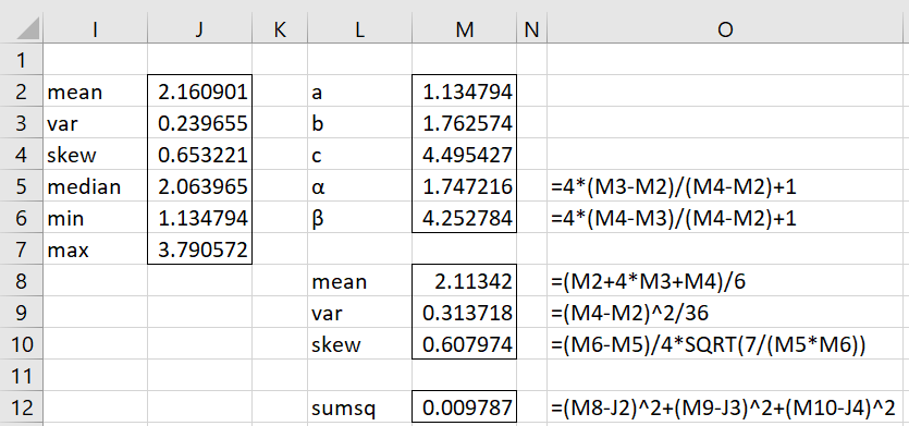
The key here is that bounds are specified for the distribution parameters. Upon clicking the Solve button, the results shown in Figure 4 are obtained.
Figure 4 – Solver results
This time, the parameters are acceptable, and the fit is pretty good (again a low sumsq), but not quite as good as in Example 1. Note too that the value of a (cell M2) is equal to the value of the smallest data element in the sample (cell J6 or cell B6 from Figure 1). As we will see in Fitting PERT Distribution via MLE, this also means that the LL value will be undefined.
Using Iterative Search
We can also estimate the parameter values by iterative search in the same manner as for the triangular distribution. For more details see PERT Method of Moments Support.
Examples Workbook
Click here to download the Excel workbook with the examples described on this webpage.
References
Rao, K. S., Viswam, N., Anjaneyulu, G. (2021) Estimation of parameters of Pert distribution by using method of moments
https://www.ijraset.com/fileserve?FID=38239
Wikipedia (2023) PERT distribution
https://en.wikipedia.org/wiki/PERT_distribution


