Basic Approach
Let m, s, w be the sample mean, standard deviation, and skewness respectively of a data set that we wish to fit a GEV distribution. Since, as described in GEV Distribution
![]()
![]()
where gk = Γ(1–kξ), assuming that we already have an estimate for ξ, we can estimate μ and σ by
![]()
![]()
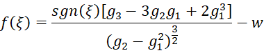
We can estimate ξ by solving the following equation which expresses the sample skewness, for ξ
![]()
In particular, we can use any of the various root-finding approaches (e.g. Newton’s or Brent’s method) to find the value of ξ which satisfies f(ξ) = 0 where
Example
Example 1: Fit a GEV distribution to the data in range A2:A51 of Figure 1 using the Method of Moments (only the first 23 elements of the data are displayed).
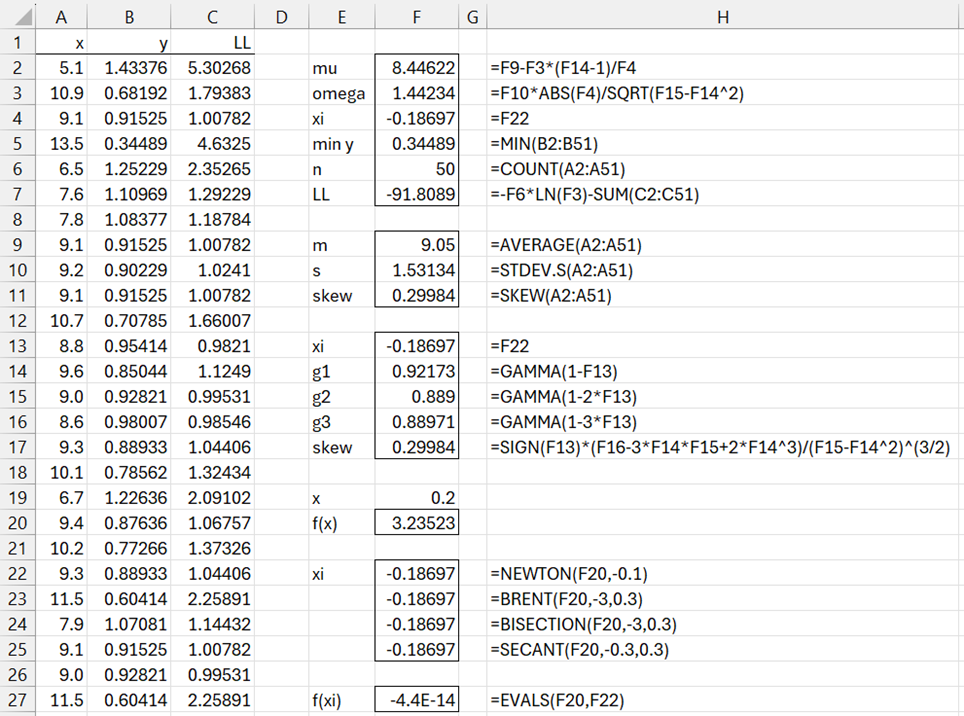
Figure 1 – Fitting data to GEV distribution
We start by calculating the skewness of the data using the formula =SKEW(A2:A51), as shown in cell F11. We now seek the value of ξ that yields the value of skewness in F11 based on the formula in cell F17 (i.e. by using the method of moments). It turns out that this value for ξ is -.18696821 as shown in cell F13.
Based on this value of ξ, we can calculate the values of g1, g2, and g3, as shown in cells F14, F15, and F16, from which we calculate the skewness shown in cell F17, and this value matches the sample skewness value shown in cell F11.
Finding ξ
But how did we obtain the value for ξ shown in cell F13? The skewness value in cell F17 is based on the ξ value in cell F13, which is the value of ξ such that f(ξ) = 0 where f(ξ) is calculated in cell F20, essentially by the formula =F17-F11. We can find this value using any of the formulas shown in cells F22 to F25, i.e. by using Newton’s method, Brent’s method, etc. for finding the root of a continuous function. That the value in cell F13 is the value of ξ for which f(ξ) = 0 is confirmed in cell F27.
As mentioned above, ideally, we would like to use the formula =F17-F11 in cell F20, but this has the problem that the formula in cell F20 contains references to cells that reference cell F13 (i.e. ξ) indirectly, which is prohibited when using the NEWTON, BRENT, BISECTION or SECANT worksheet functions (see Root Finding Functions). As a result, we need to ensure that the formula in cell F20 directly contains all references to ξ. This is accomplished by placing the following long formula in cell F20:
=SIGN(F19)*(GAMMA(1-3*F19)-3*GAMMA(1-F19)*GAMMA(1-2*F19)+2*GAMMA(1-F19)^3)/(GAMMA(1-2*F19)-GAMMA(1-F19)^2)^(3/2)-F$11
Note that the reference to cell F19 is a dummy reference to the one unknown variable x in the formula f(x). Essentially F19 is a stand-in for ξ. Also, since we used absolute addressing for F11 (via the $), the formula in cell F20 uses the value in cell F11 and doesn’t treat it like a variable.
Finally, note that we could have also found the value for ξ using Excel’s Goal Seek capability, as we have done in numerous places on the website.
Once we find the fitted value for ξ, we can obtain the values for μ and σ, as shown in cells F2 and F3.
MLE Approach
The value of the log-likelihood function based on these three parameters is shown in cell F7 using the formula described in Fitting a GEV Distribution via MLE. The formula in cell F7 references the values in column C. E.g. cell C2 contains the formula =(1+1/$F$4)*LN(B2)+B2 ^ (-1/$F$4) and cell B2 contains the formula =1+$F$4*(A2-$F$2)/$F$3.
Examples Workbook
Click here to download the Excel workbook with the examples described on this webpage.
References
Martins, E. S., Stedinger, J. R. (2000) Generalized maximum-likelihood generalized extreme-value quantile estimators for hydrologic data
https://agupubs.onlinelibrary.wiley.com/doi/10.1029/1999wr900330
https://staff.ral.ucar.edu/ericg/read2.pdf