Example
Example 1: Fit the data in A2:A16 of Figure 1 to a generalized gamma distribution using the method of moments. In particular, find the parameters of such a distribution such that the first three moments based on this distribution are as close as possible to the observed sample moments.
We are going to use the following formulas for k = 1, 2, and 3 to fit data to a generalized gamma distribution (as described in Generalized Gamma Distribution).

This is accomplished in cells D2, D3, and D4 of Figure 1. Cell D2 contains the formula =AVERAGE(A2:A16), cell D3 contains the array formula =AVERAGE(A2:A16^2), and E3 contains the array formula =AVERAGE(A2:A16^3). The formulas in column E are shown in column G.
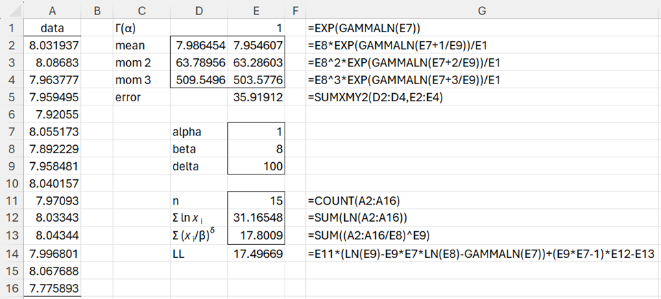
Figure 1 – Fitting a Generalized Gamma Distribution
We explain the calculation of the log-likelihood function value (in cell D14) in Fitting General Gamma Distribution Parameters using MLE.
Using Solver
Since we want to use the method of moments, we seek the values of α, β, and δ in E7:E9 so that the values in D2:D4 and E2:E4 are as close as possible. This is formalized by minimizing the value in E5 using Excel’s Solver. We do this by selecting Data > Analyze|Solver, and then filling in the dialog box that appears as shown in Figure 2.
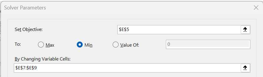
Figure 2 – Upper portion of Solver dialog box
After pressing the OK button on the dialog box, the values on the spreadsheet in Figure 1 change to those shown in Figure 3.
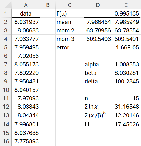
Figure 3 – Update of parameter values
We see that the new parameter values in E7:E9 result in an error value in cell E5 close to zero. Thus, we consider these values as good estimates for the generalized gamma distribution parameters.
Using Solver’s Multistart
Note, however, that the resulting parameters are highly dependent on the initial values assigned for these parameters as shown in E7:E9 of Figure 1. To partially overcome this problem, we make use of Solver’s Multistart capability. Using this capability Solver will use a variety of initial values for these parameters, and then optimize the parameters for each iteration. Solver will then return the parameter values with the smallest value in cell E5. To use the Multistart capability, a lower and upper bound must be assigned to each of the three parameters. This is done as shown in the dialog box in Figure 4.
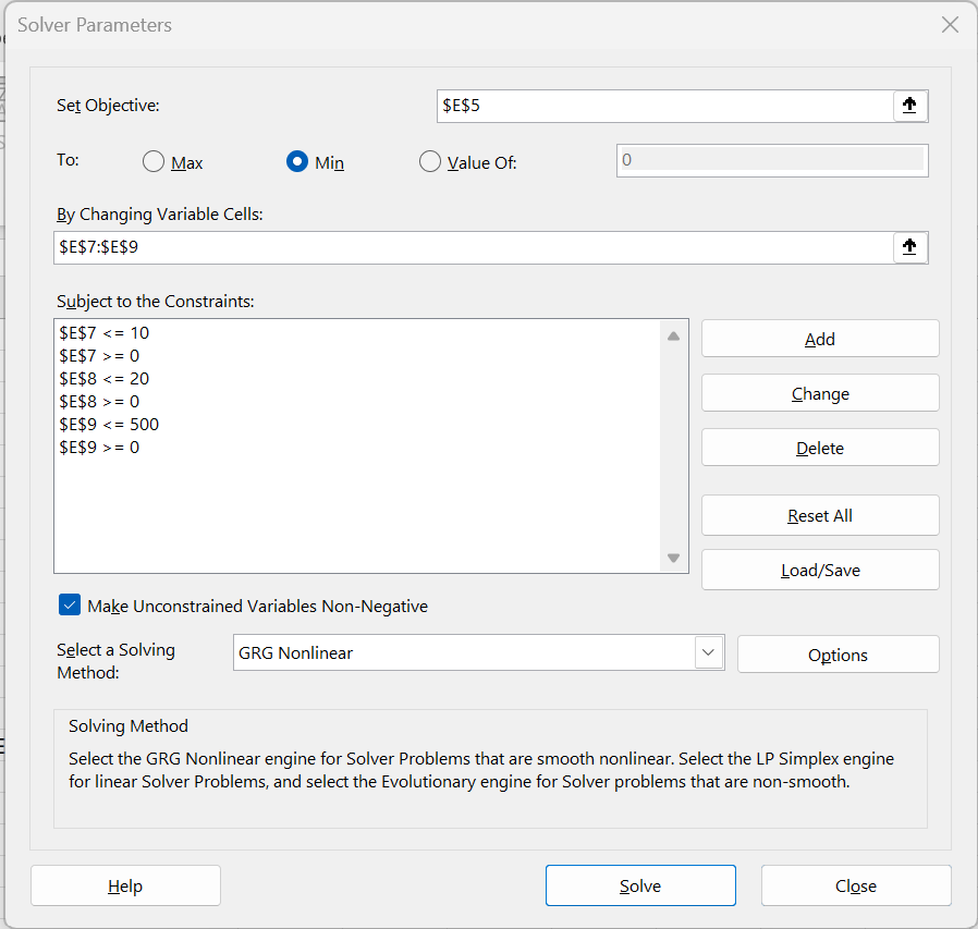
Figure 4 – Solver dialog box with constraints
Next, we click on the Options button and then click on the Use Multistart check box (on the GRG Nonlinear tab). We elect to perform 2,000 iterations by inserting the value 2,000 in the Population Size field. This time we obtain the results shown in Figure 5.
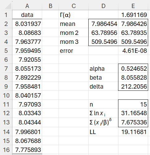
Figure 5 – Optimized results
We see from Figure 5 that the parameters in E7:E9 result in an even closer fit (i.e. the value in cell E5 is even closer to zero (than that in cell E5 of Figure 3). Note too that the log-likelihood value in cell E14 is bigger than that shown in Figure 3, which is a positive development.
Examples Workbook
Click here to download the Excel workbook with the examples described on this webpage.
References
Nematrian (2023) The generalised gamma distribution
http://www.nematrian.com/GeneralisedGammaDistribution
Jimenez Nava, V. H. (2011) Gamma and generalized gamma distributions
https://scholarworks.utep.edu/open_etd/2321/
How can i solve wakeby (5-parameter)/Log-Pearson III (3-Parameter)/Generalized Gamma (4-Parameter) distribution? Is there any built up function in realstatsexcel?
Hello Rahat,
Real Statistics does not support this distribution.
I will look into adding it in the next release.
Charles