Log-likelihood Function
The pdf of the PERT distribution for a ≤ x ≤ c is
where
Now, suppose we have a dataset x1, …, xn from the PERT distribution. The likelihood function is
Therefore, the log-likelihood function can be expressed by
Real Statistics Function: The Real Statistics Resource Pack provides the following worksheet function
PERT_MLE(R1, a, b, c): returns the log-likelihood estimate LL for the data in R1 based on a PERT distribution with parameters a, b, and c.
Fit using MLE
We can also estimate the parameter values by iterative search using the MLE approach in the same manner as we did for the method of moments. In this case, the goal is to find the PERT parameters that maximize LL instead of minimizing the sum of squares.
Real Statistics Function: The Real Statistics Resource Pack provides the following worksheet function that estimates the parameters of a PERT distribution that fits the data in R1 based on the method of moments.
PERT_FIT(R1, lab, lo, hi, iter, exta, extc, iterb, iterc): returns a column array with the estimated values of the parameters a, b, c; along with the mean, variance, and skewness based on the data in R1 and the distribution parameters; and finally, the MLE and the sum of squares.
The arguments are exactly as for PERT_FITM (see MoM Support for PERT Distribution), except there is no version where iter <= 0.
Observation: Note that you can also use Solver, but in this case, you must use initial guesses that are close to the optimum parameter values. E.g. if your initial guesses are 1.1, 2.0, 3.8, then Solver will converge to a solution, but if your initial guesses are 1.0, 2.0, 3.8, then it won’t.
Example
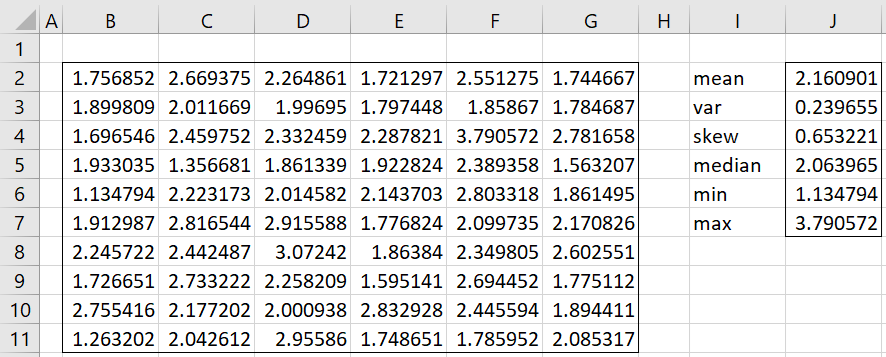
Example 1: Fit the data in range B2:G11 of Figure 1 to a PERT distribution using the MLE approach.
Figure 1 – Fitting a PERT distribution
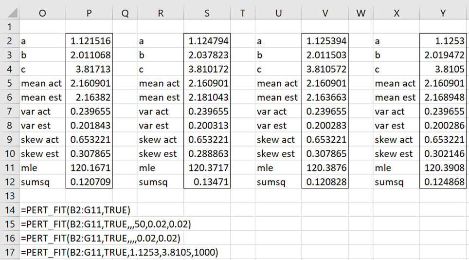
We use the formula =PERT_FIT(B2:G11,TRUE) in O2:P12 of Figure 2. The default value for exta and extc are used, namely
exta = extc = (max – min)/2 = (3.790572 – 1.134794)/2 = 1.327889
Also, since iter defaults to 100, the values of a and c are searched in increments of 1.327889/100 = .01327889 in the ranges
-.1931 = 1.134794 – 1.327889 = min – exta ≤ a < min = 1.134794
3.790572 = max < c ≤ max + extc = 3.790572 + 1.327889 = 5. 118461
Figure 1 – Fitting a PERT distribution via MLE
In the second application of PERT_FIT, namely =PERT_FIT(B2:G11,TRUE,,,50,.02,.02), we restrict the range of a and c to
1.114794 ≤ a <1.134794 3.790572 < c ≤ 3.810572
which includes the values a = 1.121516 (cell P2) and c = 3.81713 from the first application of PERT_FIT. Even though we use a smaller number of iterations, namely 50, the function uses a finer search since increments of .02/50 = .0001 are employed. We see that indeed MLE increases from 120.1671 to 120.3717.
In the third application, we again use the default iter of 100, and see that MLE increases to 120.3876. The processing of this case is slower than the previous one (by a factor of about 2^3 = 8).
Finally, in the last example, we set a = 1.1253 and c = 3.8105. Thus, the function only needs to search for the value of b. We use iter = 1,000 to obtain a slightly better value of MLE, namely MLE =120.3908. This case is much faster than the previous one since there are 1,000 iterations instead of 100 × 100 × 100 = 100,000.
Examples Workbook
Click here to download the Excel workbook with the examples described on this webpage.
References
Rao, K. S., Viswam, N., Anjaneyulu, G. (2021) PERT distribution and its properties.
https://www.irjmets.com/uploadedfiles/paper/volume_3/issue_10_october_2021/16799/final/fin_irjmets1635145380.pdf
Rao, K. S., Viswam, N., Anjaneyulu, G. (2021) Estimation of parameters of PERT distribution by using maximum product of spacings method
https://ijcrt.org/papers/IJCRT2109281.pdf


