Fitting triangular dist via MLE| Real Statistics Using Excel

Log-likelihood Function

Suppose that we have a sample x₁, x₂, …, x_n from a triangular distribution with parameters a, b, c. Let’s also suppose that the data elements are in sorted order x₁ ≤ x₂ ≤ … ≤ x_n.

Since the pdf of the triangular distribution for a ≤ x ≤ c is

the likelihood function is given by

where r is an index such that

where x₀ = a and x_n₊₁ = c. It follows that

Thus, the log-likelihood function is

As shown in Kotz and van Dorp, the maximum value of LL is achieved when b = x_r for some r = 1, 2, …, n. Thus, we can choose values of a < x₁ and c > x_n, but once these values are chosen, b is restricted to x₁, .., x_n.

Worksheet Functions

Real Statistics Functions: The Real Statistics Resource Pack provides the following worksheet functions for the data in R1.

TRIANG_MLE(R1, a, b, c) = LL for a triangular distribution with parameters a, b, and c which fits the data in array R1.

TRIANG_FIT(R1, lab, lo, hi, iter, exta, extc, iterc): returns a column array with the estimated values of the parameters a, b, c; along with the mean, variance, and skewness based on the data in R1 as well as based on the distribution parameters; and finally the MLE and the sum of squares.

If lab = TRUE (default FALSE), then a column of labels is appended to the output.

If lo is present, then a is set to lo; otherwise, a is calculated using the MLE. If hi is present, then c is set to hi; otherwise, c is calculated using MLE.

Improving the estimates

If lo is missing, then the function assumes that a is in the range

mn – exta ≤ a < mn

where mn is the smallest element in R1. In particular, the function tests a₁, a₂, …, a_k as potential values for a where k = iter, and

a₁ = mn – exta a_i₊₁ = a_i + exta/iter

Similarly, if hi is missing, then the function assumes that c is in the range

mx < c ≤ mx + extc

where mn is the smallest element in R1. In particular, the function tests c₁, c₂, …, c_h as potential values for c where h = iterc, and

c₁ = mx + extc c_i₊₁ = c_i – extc/iterc

If exta is missing, then it defaults to (mx – mn)/2. When extc is missing, then it defaults to the value of exta. If iter is missing, it defaults to 100. If iterc is missing it defaults to the value of iter.

Finally, for every combination of a and c, as described above, the function tests the values x₁, x₂, …, x_n in R1 as potential values for b (for these a and c values).

If lo and hi are specified, then a and c are defined, and so only b needs to be estimated; this requires iter iterations. If neither hi nor lo is specified, then all three parameters need to be specified; this requires iter³ iterations (which is 1,000,000 for the default value of iter). When hi or lo is specified, but not both, then iter² iterations are required (10,000 for the default value of iter).

Comparison of moments

For TRIANG_FIT, MLE is the maximum LL value for the data in R1; the goal is to determine the a, b, and c values that maximize this value.

For a triangular distribution, the mean, variance, and skewness can be calculated via the following formulas (see Triangular Distribution).

The corresponding sample values m, v, and w can be calculated from the data in R1 via the formulas =AVERAGE(R1), =VAR.S(R1), and =SKEW(R1). We set sumsq equal to

(mean – m)² + (var – v)² + (skew – w)²

The smaller the value of sumsq, the better the fit.

Example when all parameters are unknown

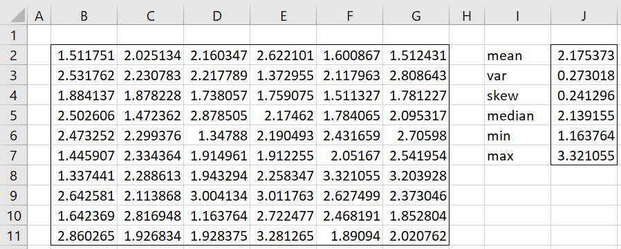
Example 1: Fit the data in range B2:G11 of Figure 1 to a triangular distribution using MLE (i.e. by maximizing LL).

Figure 1 – Fitting data to triangular distribution by MLE (part 1)

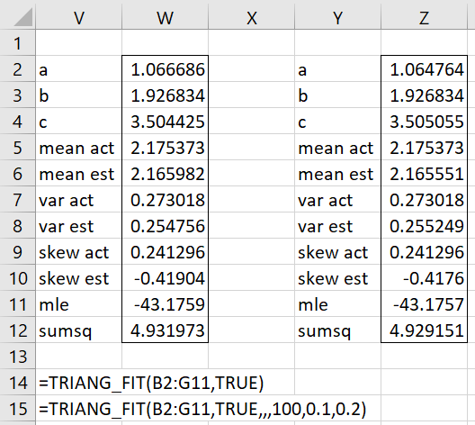
We use the formula =TRIANG_FIT(B2:G11,TRUE) to obtain the results shown in V2:W12 of Figure 2.

Figure 2 – Fitting data to triangular distribution by MLE (part 2)

If we want to improve the accuracy of our estimates, we can increase the value of iter or reduce the intervals used to find a and c. We show how to do the latter.

Improving accuracy

As described above, the formula tests values of a and c in the ranges

mn – exta ≤ a < mn mx < c ≤ mx + extc

Since exta and extc default to (mx–mn)/2 = (3.321055 – 1.163764)/2 = 1.07864. These ranges are 1.0864 wide. In fact, the value for a in cell W2 is only 1163764 – 1.066686 = .097078 from the minimum data value. Similarly, c in cell W4 is only 3.504425 – 3.321055 = .18337 away from the maximum value. Thus, we can actually use exta = .097078 and extc = .18337. Since these will produce much smaller ranges, we should get more accurate results. Just to be safe, we’ll choose slightly wider ranges where exta = .1 and extc = .2 by using the formula =TRIANG_FIT(B2:G11,TRUE,,,,.1,.2).

This means that we have reduced the interval for a by a factor of more than 10 and the interval for c by a factor of more than 5, for a 50-fold improvement. We would need to increase iter to 1000 and iterc to 500 to get a similar improvement (at the cost of much slower processing time). The result is shown in Y2:Z12 of Figure 2. The improvement is pretty minor: the MLE value is only .0002 higher.

Finally, while this approach maximizes MLE. The resulting skewness (cell W10) is not consistent with the skewness of the sample (cell W9). As expected, the method of moments will bring these estimates more in line with the sample values. As we see in MoM: Triangular Distribution (under construction), the LL resulting from the method of moments (-43.4102) is only slightly lower than that found above (-43.1759), and so for this example, the MoM seems to give a better fit.

Examples when some parameters are known

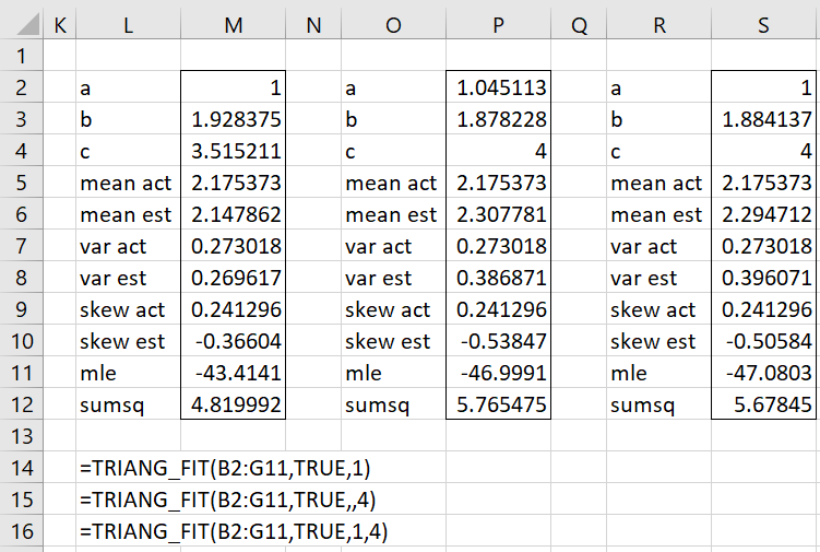
Example 2: (a) Suppose we know that for the data in Figure 1, a = 1. Find the values of b and c that maximize MLE. (b) Suppose we know that c = 4, find the values of a and b that maximize MLE, Finally, (c) suppose we know that a = 1 and c = 4, find the value of b that maximizes MLE.

The results are shown in Figure 3.

References

Cook, J. (2015) Fitting a triangular distribution
https://www.johndcook.com/blog/2015/03/24/fitting-a-triangular-distribution/#:~:text=One%20way%20to%20fit%20a,if%20these%20values%20are%20known.
Stack Exchange (2016) MLE for triangular distribution
https://stats.stackexchange.com/questions/64102/mle-for-triangle-distribution/64103#64103
Kotz, S., van Dorp, R.(2004) The triangular distribution. Beyond Beta
https://books.google.it/books/about/Beyond_Beta_Other_Continuous_Families_Of.html?id=JO7ICgAAQBAJ&redir_esc=y