One of the goals of the Taguchi approach is to optimize the early stages of product or system design, especially by reducing the number of experiments or trials that need to be conducted. Here the goal is to extract as much information as possible for the least cost (in terms of time, resources, and money). The approach uses a small number of standard orthogonal arrays and fits the design to one of these arrays.
2-level Design Overview
In particular, we consider the fractional 2^k designs described in Figure 1. These designs are limited to two levels, which are labelled 1 and 2 (instead of -1 and 1 as in 2^k Factorial Design ).
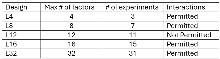
Figure 1 – Two-level designs
See List of 2-level Designs and Interactions to see all these designs.
Since we want to reduce costs, we limit our analysis to main effect factors or at most the interaction between two factors. An example of an L8 design is shown in Figure 2.
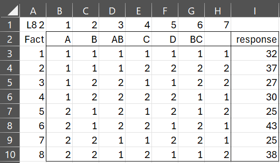
Figure 2 – L8 Design
The core of an L8 design, shown in range B3:H10, contains 7 columns, one per a maximum of 7 factors and 8 rows, one per trial. This part of the design is fixed and always contains the same sequence of 1’s and 2’s.
Each column in the design is headed by a factor label (in range B2:H2). We use a one-character symbol to represent a main factor and a two-character symbol to represent an interaction between two factors. You can place the main factor labels anywhere in row 2 but there are restrictions as to where interaction symbols can be placed, as described below. In addition, you can optionally leave some column labels blank.
You also need to provide the numeric output for each trial, as shown in range I3:I10. Only numerical values can appear in the response column. You can also add additional response columns if you had replications for each of the trials.
Example
Example 1: Use Taguchi’s L8 design to determine how best to sound-proof a new air-conditioning unit. We address the 4 factors shown in Figure 3 plus the interaction between factors A and B, and between B and C.
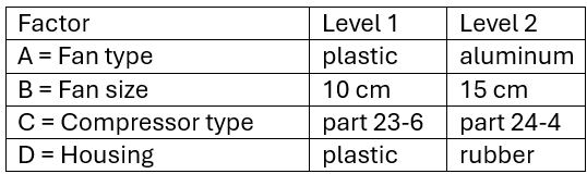
Figure 3 – Factors and levels
We now run the 8 trials described in Figure 2 to obtain the noise levels listed in range I3:I10. E.g. in the trial (row 8) where we use an aluminum fan of size 15 cm, a part 23-6 compressor and rubber housing, we observed a noise level of 38.
ANOVA Model
We now use ANOVA to determine which of the factors plays a large enough role in the design and which are less important. The results are shown in Figure 4.
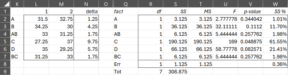
Figure 4 – ANOVA
On the left side of the figure are the averages for each of the factor × level combinations. E.g. cell M3 contains the mean result for level 2 of Factor B. This can be obtained by identifying all the rows with a 2 in the second column (for factor B) and taking the average in the results column for these rows, namely (27 + 30 + 25 + 38) / 4 = 30.
In general, the values in columns L and M can be filled in by inserting the following formula in cell L2, highlighting range L2:M7, and pressing Ctrl-R and Ctrl-D.
=IFERROR(AVERAGEIF(INDEX($B$3:$H$10,,MATCH($K2,$B$2:$H$2,0)),L$1,$I$3:$I$10),””)
The delta values are simply the difference between the level 1 and level 2 values for each factor.
We can now fill in the ANOVA table on the right of Figure 3 by observing that the df for each factor is 2-1 = 1. Since there are 8 rows dfTot = 8-1 = 7 and dfErr = 1, as calculated by the formula =R9-SUM(R2:R7).
The sum of squares for factor A (SSA) is calculated via the formula =DEVSQ(L2:M2), i.e. .78125, times the number of times each of the levels is repeated in any column, namely 4. SSA = .78125 × 4 = 3.125, as shown in cell S2. In general, we can use the following formula:
=DEVSQ(L2:M2)*COUNTIF(INDEX($B$3:$H$10,,MATCH(Q2,$B$2:$H$2,0)),1)
As usual, SSTot is calculated by the formula =DEVSQ(I3:I10) and SSErr by =S9-SUM(S2:S7).
SS% column
We fill in the rest of the table as for any ANOVA, adding a SS% column, which is simply the percentage of the total sum of squares accounted for by each factor. E.g. cell W2 contains the formula =S2/S9.
We see that factors A, AB, and BC have low SS% values, namely 1.01%, 1.98%, and 1.98%. A rough rule-of-thumb is that values under 10% are generally considered to be low. We could also use the p-value as a rough guide.
Note that if we had a fifth factor E (in cell H2 of Figure 2), then we would have a saturated design, and so dfErr and SSErr would be zero. In this case most of the ANOVA table would consist of error values, including the p-values. We could still use the SS% column to indicate which factors are not making an important contribution to the design.
Dropping less important factors
If we eliminate factors A, AB, and BC from the design, we obtain the revised design shown in the bottom part of Figure 5.
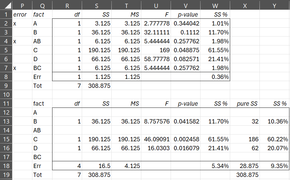
Figure 5 – Revised ANOVA
Here, the contributions of the factors being eliminated are added to the error term. E.g. cell S18 contains the formula =S8+S2+S4+S7, or more simply, =S19-SUM(S12:S17). The pure SS are calculated from the SS values. E.g. X13 contains the formula =S13-R13*T$18 and X18 contains the formula =X19-SUM(X12:X17).
Efficiency of Taguchi designs
A full factorial experiment with 7 factors requires 27 = 128 test runs. Taguchi’s L8 design supports a fractional factorial experiment with only 8 test runs.
Continuation
We continue with a description of 2-level Taguchi designs (using Example 1) on the following webpages:
- Design optimization
- List of 2-level designs and interactions
- Data analysis tool and worksheet functions
- Design with replications
- Signal-to-noise ratio
Examples Workbook
Click here to download the Excel workbook with the examples described on this webpage.
References
Roy, R. K. (2010) A primer on Taguchi method. 2nd ed. Society of Manufacturing Engineers
https://www.scribd.com/document/381615601/288020391-a-Primer-on-the-Taguchi-Method
University of York (2004) Orthogonal arrays (Taguchi designs)
No longer available online
Minitab (2024) Catalogue of Taguchi designs
https://support.minitab.com/en-us/minitab/help-and-how-to/statistical-modeling/doe/supporting-topics/taguchi-designs/catalogue-of-taguchi-designs/
Kacker, R. N., Lagergren, E. S. and Filliben, J. J. (1991) Taguch’s orthogonal arrays are classical designs of experiments. J. Res. Natl. Inst. Stand. Technol. 96, 577
https://www.ncbi.nlm.nih.gov/pmc/articles/PMC4927234/pdf/jresv96n5p577_a1b.pdf