Fractional 2^k Designs

Basic Concepts

In a design with k factors, you need to perform at least 2^k measures (even without replications). This can sometimes be time-consuming or expensive. In these cases, fractional factorial design can be useful.

In this approach, we confound some factors with higher order interactions of other factors (which are assumed to be non-significant). E.g. in a 2^4 design with factors A, B, C and D we would typically need 2^4 = 16 data elements. We can instead use a 2^(4-1) fractional design containing 8 data elements. Here we confound factor D with factor ABC since we can usually assume that interactions of degree three are not significant.

Example

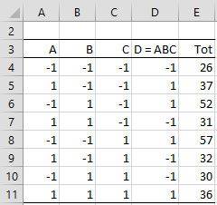
Example 1: Determine which factors are most important based on the data in Figure 1.

Figure 1 – Data for a 2^(4-1) design

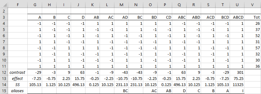
Note that any factor squared is equivalent to I, a column vector of all ones. Thus, confounding D with ABC results in other interactions being confounded. E.g. AD = AABC = A²BC = IBC = BC. Thus AD and BC are confounded. Similarly, ACD = ACABC = BA²C² = B, which means that B is confounded with ACD (aka B is an alias for ACD). Since interactions of degree three such as ACD are generally not significant, this shouldn’t cause problems. That interactions of degree 2, such as AD and BC, are confounded usually is important and so we need to look at such factors combined, i.e. AD+BC.

We capture these facts in Figure 2.

Figure 2 – Fractional 2^(4-1) design

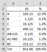
From Figure 2, we obtain the variation summary shown in Figure 3.

Figure 3 – Variation by factor

Note that the sum of the SS values, 853.88, shown in cell Y10, can also be calculated by =DEVSQ(E4:E11). We see from Figure 3 that factors A, D, and BC account for most of the variation in this design and should be the focus of any more detailed follow-up design. Fortunately, for this example, the confounding of two-level interactions was not much of a problem. This won’t always be the case.

Optimal Assignments

Note that there are multiple ways of confounding factors. For Example 1, we could have confounded D with AB instead of ABC. A rule of thumb, however, is to choose confounding with the highest levels of interaction possible. Two simple factors (e.g. A and D) should never be confounded and confounding with interactions of degree 2, such as in Example 1, should be avoided, although this won’t always be possible.

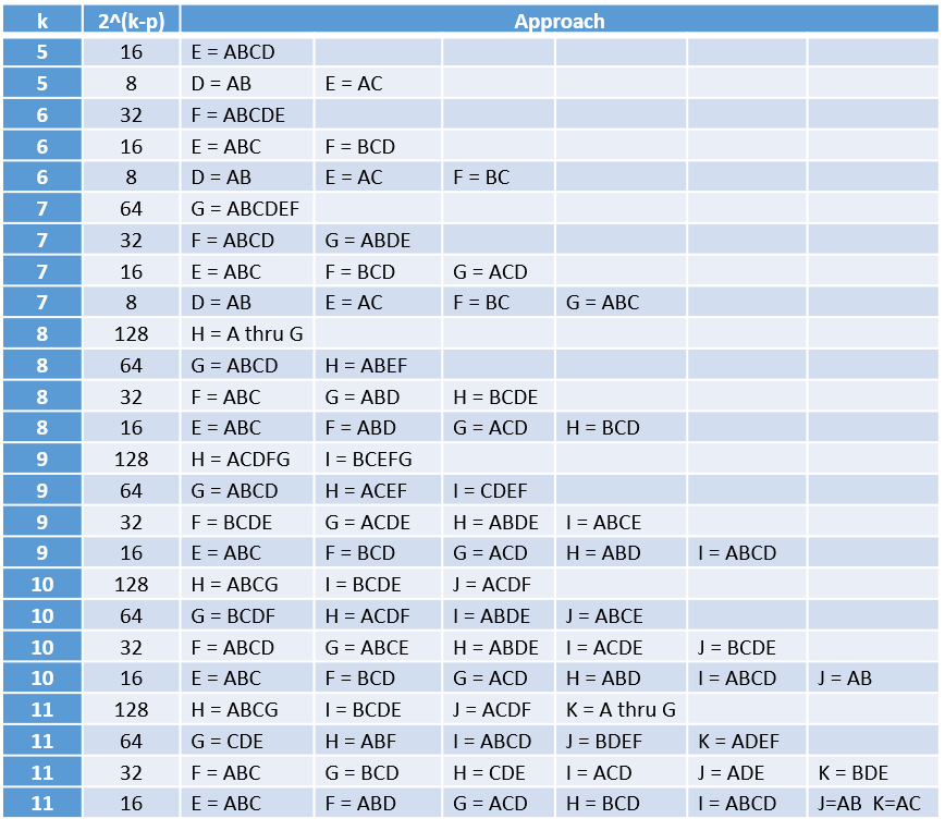
In Example 1 we halved the number of samples required from 16 to 8. It is also possible to perform multiple confounding to reduce the sample size by a multiple of 2, 4, or even more. Figure 4 shows optimal assignments.

Figure 4 – Confounding assignments

Examples Workbook

Click here to download the Excel workbook with the examples described on this webpage.

References

PennState (2017) Blocking and confounding in the 2^k factorial design
https://online.stat.psu.edu/stat503/lesson/7

PennState (2017) 2-level fractional factorial design
https://online.stat.psu.edu/stat503/lesson/8

Montgomery, D. C. (2012) Blocking and confounding in the 2^k factorial design. Design and analysis of experiments, 8th ed.
https://faculty.ksu.edu.sa/sites/default/files/douglas_c._montgomery-design_and_analysis_of_experiments-wiley_2012_edition_8.pdf