Classification Table

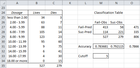
A Classification Table (aka a Confusion Matrix) describes the predicted number of successes compared with the number of successes actually observed. Similarly, it compares the predicted number of failures with the number actually observed.

Possible Outcomes

We have four possible outcomes:

True Positives (TP) = the number of cases that were correctly classified to be positive, i.e. were predicted to be a success and were actually observed to be a success

False Positives (FP) = the number of cases that were incorrectly classified as positive, i.e. were predicted to be a success but were actually observed to be a failure

True Negatives (TN) = the number of cases that were correctly classified to be negative, i.e. were predicted to be a failure and were actually observed to be a failure

False Negatives (FN) = the number of cases that were incorrectly classified as negative, i.e. were predicted to be a failure but were actually observed to be a success

Classification Table

The corresponding Classification Table takes the form

where PP = predicted positive = TP + FP, PN = predicted negative = FN + TN, OP = observed positive = TP + FN, ON = observed negative = FP + TN and Tot = the total sample size = TP + FP + FN + TN.

Example 1: Researchers are testing a new spray for killing mosquitoes. In particular, they want to discover the correct dosage of the spray. They tested 806 mosquitoes with dosages varying from 0 μg to 20 μg. They then tabulated the number of mosquitoes who died and lived in 2 μg dosage intervals. These results are displayed in range A24:C34 of Figure 1.

Create a classification table for a dosage of 10 μg or more. The researchers view success as the mosquito died and failure as the mosquito lived. They viewed a dosage of lower than 10 μg as a prediction of failure (mosquito lives) and a dosage of 10 μg or more as a prediction of success (mosquito dies).

Figure 1 – Classification Table

We decide to set the cutoff value to the 5th row (8.00 – 9.99) as shown in cell M33. 

For the data in Figure 1 we have

TN = 413 (cell M27), which can be calculated by the formula =SUM(B25:B29)

FN = 58 (cell N27), which can be calculated by the formula =SUM(C25:C29)

FP = 114 (cell M28), which can be calculated by the formula =B35-M27

TP = 221 (cell N28), which can be calculated by the formula = C35-N27

Relative Statistics

We now can define the following:

True Positive Rate (TPR), aka Sensitivity = TP/OP = 221/279 = .792115 (cell N31)

True Negative Rate (TNR), aka Specificity = TN/ON = 413/527 = .783681 (cell M31)

Accuracy (ACC) = (TP + TN)/Tot = (221+413) / 806 = .7866 (cell O31)

False Positive Rate (FPR) = 1 – TNR = FP/ON = 114/527 = .216319

Positive Predictive Value (PPV) = TP/PP = 221/335 = .659701

Negative Predictive Value (NPV) = TN/PN = 413/471 = .876858

Accuracy is a measure of the fit of the model (i.e. a dosage of 10 μg or more in this example). For Example 1 this is .7866, which means that the model gives an accurate prediction 78.66% of the time, or simply stated 78.66% of the mosquitoes show the right outcome: they die when the dosage is 10 μg or more and live when the dosage is less than 10 μg.

Note that FPR is the type I error rate α and FNR is the type II error rate β as described in Hypothesis Testing. Thus, sensitivity is equivalent to power 1 – β.

Examples Workbook

Click here to download the Excel workbook with the examples described on this webpage.

References

Wikipedia (2014) Confusion matrix
https://en.wikipedia.org/wiki/Confusion_matrix

IBM SPSS (2016) Classification table
https://www.ibm.com/docs/en/spss-statistics/24.0.0?topic=model-classification-table