Ranking Functions in Excel

Basic Concepts

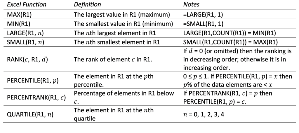
Excel Functions: Figure 1 summarizes the various ranking functions available in all versions of Excel for a data set R1. We describe each of these functions in more detail on the rest of this webpage, plus we describe additional ranking functions that are only available in versions of Excel starting with Excel 2010.

Figure 1 – Ranking functions in Excel

All these functions ignore any empty cells and cells with non-numeric values.

MIN and MAX

Definition 1: MIN(R1) = the smallest value in R1 and MAX(R1) = the largest value in R1

Example 1: For range R1 with data elements {4, 0, -1, 7, 5}

• MIN(R) = -1
• MAX(R) = 7

SMALL and LARGE

Definition 2: SMALL(R1, n) = nth smallest value in R1 and LARGE(R1, n) = nth largest value in R1. Here n can take on any value from 1 to the number of elements in R1, i.e. COUNT(R1).

Observation:

SMALL(R1, n) = LARGE(R1, COUNT(R1) – n + 1)

LARGE(R1, n) = SMALL(R1, COUNT(R1) – n + 1)

Example 2: For range R1 with data elements {4, 0, -1, 7, 5}

• LARGE(R1, 1) = 7, LARGE(R1, 2) = 5, LARGE(R1, 5) = -1
• SMALL(R1, 1) = -1, SMALL(R1, 2) = 0, SMALL(R1, 5) = 7

Real Statistics Function: The Real Statistics Resource provides the following worksheet function.

SMALLExact(R1, k): When k is an integer, this function is equivalent to SMALL(R1,k). Otherwise, it takes the interpolated value =SMALL(R1,INT(k))+(k-INT(k))*(SMALL(R1,INT(k)+1)-SMALL(R1,INT(k)))

RANK

Definition 3: RANK(c, R1, d) = the rank of data element c in R1. If d = 0 (or is omitted) then the ranking is in decreasing order, i.e. a rank of 1 represents the largest data element in R1. If d ≠ 0 then the ranking is in increasing order and so a rank of 1 represents the smallest element in R1.

Example 3: For range R1 with data elements {4, 0, -1, 7, 5}

• RANK(7, R1) = RANK(7, R1, 0) = 1
• RANK(7, R1, 1) = 5
• RANK(0, R1) = RANK(0, R1, 0) = 4
• RANK(0, R1, 1) = 2

Observations

• If LARGE(R1, n) = c then RANK(c, R1) = RANK(c, R1, 0) = n
• If SMALLR1, n) = c then RANK(c, R, 1) = n
• RANK(c, R1) + RANK(c, R1, 1) = COUNT(R1) + 1
• For any values c and d, 1 ≤ RANK(c, R1, d) ≤ COUNT(R1)

Excel’s RANK function does not take care of ties very well. E.g., if the range R1 contains the values {1, 5, 5, 0, 8}, then RANK(5, R1) = 2 because 5 is the 2^nd highest ranking element in range R. But 5 is also the 3^rd highest ranking element in the range, and so for many applications, it is useful to consider the ranking to be 2.5, namely the average of 2 and 3.

To correct for ties for any data element c in the range R1, you can use the following formula (see Built-in Excel Functions for a description of the COUNTIF function):

= RANK(c, R1) + (COUNTIF(R1, c) – 1) / 2

Excel Worksheet Functions

Excel addresses this issue by providing the function RANK.AVG, which takes the same arguments as RANK but returns the average of equal ranks as described above. Excel also provides the function RANK.EQ, which is equivalent to RANK.

While the RANK function is available in all releases of Excel, the RANK.AVG and RANK.EQ functions are not available in releases prior to Excel 2010.

If the range R1 contains the values {1, 5, 5, 0, 8}, then RANK.AVG(5, R1) = 2.5, while if R1 contains the values {1, 5, 5, 8, 5}, then RANK.AVG(5, R1) = 3, i.e. the average of 2, 3, and 4.

Real Statistics Functions

For users of versions of Excel prior to Excel 2010, the Real Statistics Resource Pack provides the function RANK_AVG which is equivalent to RANK.AVG. In fact, as explained below, RANK_AVG has some advantages over RANK.AVG even for users of newer versions of Excel.

RANK_AVG(x, R1, order, num_digits) = the ranking of x in range R1, where x, as well as any numeric entries in R1, are rounded off to num_digits decimal places; when there are ties, the average ranking is used. If num_digits is omitted then it defaults to 8. If order = 0 (or is omitted) then the ranking is in decreasing order, while if order ≠ 0 then the ranking is in increasing order.

The Real Statistics Resource Pack also supplies the following related array functions:

RANKS(R1, order, num_digits): returns a column array with the values RANK_AVG(x, R1, order, num_digits) for each numeric element x in R1. Entries for non-numeric elements are not included in the list.

RANKCOL(R1, order, num_digits): returns an array of the same size and shape as R1, each column of which contains the ranks for that column (the data in each column is ranked separately).

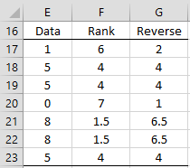
Example 4: Using the RANK.AVG or RANK_AVG function, find the ranks of the data in range E17:E23 of Figure 2.

Figure 2 – Average ranking

The result is shown in column F of Figure 2. For example, the average rank of 8 (cell E21 or E22) is 1.5, as calculated using the formula =RANK_AVG(E21,E17:E23) or =RANK.AVG(E21,E17:E23) as shown in cell F21 (or F22). If instead, you want the ranking in the reverse order (where the lowest value gets rank 1) then the results are shown in column G. This time using either =RANK_AVG(E21,E17:E23,1) or =RANK_AVG(E21,E17:E23,1) we see that the rank of 8 is 6.5 as shown in cell G21.

Cautions

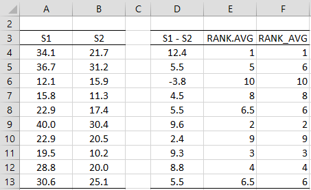
There are several flaws in the RANK, RANK.EQ and RANK.AVG functions. E.g. in Figure 3, we show two samples of data in columns A and B, with the differences shown in column D (e.g. cell D4 contains the formula =A4-B4).

Note that three cells (D5, D8, and D13) all have the value 5.5. Thus, we would expect that the rankings for each would be the same. In fact, we see that cell E5 contains the value 5 based on the formula =RANK.AVG(D5,D4:D13), while cells E8 and E13 contain the ranking 6.5. The ranking in all three cells should actually be 6. The reason for this is that apparently, the RANK.AVG function treats the value in cell D5 as slightly higher than 5.5. This produces unpredictable results.

Note too that cell E4, which contains the formula =RANK.AVG(D4,D4:D13), has the correct value, namely 1, but the formula =RANK.AVG(12.4,D4:D13) yields the error value #N/A. This means that the RANK.AVG function does not recognize 12.4 as one of the values in range D4:D13, since it doesn’t recognize the value in cell D4 as being 12.4.

Figure 3 – RANK.AVG vs. RANK_AVG

Note too that the RANK, RANK.EQ and RANK.AVG functions only take a cell range as their second argument. Thus, you can’t use an array formula such as =RANK.AVG(A4,A4:A13-B4:B13). Although A4:A13-B4:B13 evaluates to an array, it can’t be used as an argument in RANK.AVG. The Real Statistics array formula =RANK_AVG(A4,A4:A13-B4:B13), however, is valid. Keep in mind that this is an array formula, and so you must press Ctrl-Shft-Enter (unless you are using Excel 365).

In fact, you can also insert the array formula =RANK_AVG(D4:D13,D4:D13) in range F4:F13 to get the same result shown in Figure 3.

Data Analysis Tool

Excel Data Analysis Tool: In addition to the functions described above, Excel also provides a Rank and Percentile data analysis tool. This tool uses the Excel 2007 definitions of rank and percentile, i.e. those used by the RANK and PERCENTILE functions.

Example 5: Calculate the rank and percentile for the data in Figure 4 using Excel’s Rank and Percentile data analysis tool.

Figure 4 – Score data

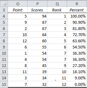
For the data in Figure 4, the data analysis tool generates the output shown in Figure 5.

Figure 5 – Rank and Percentile data analysis tool

The table is sorted in rank order. Point indicates the index of the corresponding score in the input data range. E.g. 94 (cell P4) is the 5^th data element in the input range but is the largest data element and so has rank 1.

PERCENTILE

Definition 4: For any percentage p, i.e. a value such that 0 ≤ p ≤ 1 or equivalently 0% ≤ p ≤ 100%, the worksheet function PERCENTILE(R1, p) = the element at the pth percentile.

If p(n–1) = k for some integer value k = 0, 1, 2, … n–1 where n = COUNT(R), then PERCENTILE(R1, p) = SMALL(R1, k+1) = the k+1^th element in R1. If p(n-1) is not an integer, then the PERCENTILE function performs a linear interpolation as described in the examples below.

Example 6: For range R1 with data elements {4, 0, -1, 7, 5}, the 5 data elements in R1 divide the range into 4 intervals of size 25%, i.e. 1/(5-1) = .25. Thus

• PERCENTILE(R1, 0) = -1 (the smallest element in R1)
• PERCENTILE(R1, .25) = 0 (the second smallest element in R1)
• PERCENTILE(R1, .5) = 4 (the third smallest element in R1)
• PERCENTILE(R1, .75) = 5 (the fourth smallest element in R1)
• PERCENTILE(R1, 1) = 7 (the fifth smallest element in R1)

For other values of p we need to interpolate. For example

• PERCENTILE(R1, .45) = 0 + (4 – 0) * (0.45 – 0.25) / (.5 – 0.25) = 3.2
• PERCENTILE(R1, .80) = 5 + (7 – 5) * (0.8 – 0.75) / (1.0 – 0.75) = 5.4

Of course, Excel’s PERCENTILE function calculates all these values automatically without you having to figure things out.

Excel Worksheet Functions

Releases of Excel after Excel 2007 provide two versions of the percentile function: PERCENTILE.INC and PERCENTILE.EXC. The first of these is called the inclusive version since 0 ≤  p ≤ 1, and is equivalent to PERCENTILE. The second of these is called the exclusive version of the percentile function since 0 <  p < 1.

If n = COUNT(R1), then for any integer k with 1 ≤ k ≤ n,

PERCENTILE.EXC(R1, k/(n+1)) = SMALL(R1, k), i.e. the kth smallest element in R1

For 0 < p < 1, if p(n+1) is not an integer, then PERCENTILE.EXC(R1, p) is calculated by linear interpolation between the corresponding values in R1. For p < 1/(n+1) or p > n/(n+1), no interpolation is possible, and so PERCENTILE.EXC(R1, p) returns an error value.

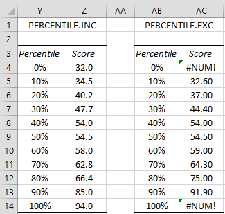
Example 7: Find the 0 – 100 percentiles in increments of 10% for the data in Figure 4 using both PERCENTILE.INC and PERCENTILE.EXC.

The result is shown in Figure 6. E.g. the score at the 60th percentile is 58 (cell Z10) using the formula =PERCENTILE.INC(B3:M3,Y10), while it is 59 (cell AC10) using the formula =PERCENTILE.EXC(B3:M3,AB10).

Figure 6 – PERCENTILE.INC vs. PERCENTILE.EXC

Real Statistics Function

The Real Statistics Resource Pack contains the following function which calculates the p^th percentile (0 ≤ p ≤ 1) based on range R1 with n elements using one of the Hyndman-Fan definitions of percentile as determined by argument m.

PERCENTILE_EXC(R1, p, m) = x_h′ + (x_h′+1 – x_h′)(h – h′)

where h′ = INT(h)  and h is defined as follows

h = np if m = 4

h = np + .5 if m = 5

h = (n+1)p if m = 6 (default)

h = (n–1)p + 1 if m = 7

h = (n+1/3)p + 1/3 if m = 8

although if this calculation results in a value smaller than the smallest value in R1 or larger than the largest value in R1, then PERCENTILE_EXC(R1, p, m) = MIN(R1) or = MAX(R1), respectively, instead of the values defined above.

PERCENTILE_EXC also supports the discontinuous Hyndman-Fan versions of percentile (where m = 1, 2, or 3).

For users of versions of Excel before Excel 2010, PERCENTILE_EXC can be used in place of PERCENTILE.EXC; in fact, PERCENTILE_EXC(R1, p) = PERCENTILE.EXC(R1, p) except when PERCENTILE_EXC(R1, p) takes an error value, in which case, PERCENTILE_EXC(R1, p) takes the value MIN(R1) or MAX(R1).

Note too that PERCENTILE_EXC(R1, p, 7) = PERCENTILE(R1, p).

Weighted Percentiles

Click here for information about weighted percentiles.

Harrell-Davis Quantiles

Another approach to calculating the percentile based on a sample is given by the Harrell-Davis Quantile. Click here for more information about this statistic.

PERCENTRANK

Definition 5: PERCENTRANK(R1, c) = the percentile of data elements in R1 up to c. Thus, if PERCENTRANK(R1, c) =  p then PERCENTILE(R1, p) = c.

Example 8: For range R1 with data elements {4, 0, -1, 7, 5}

• PERCENTRANK(R1, 5) = .75
• PERCENTRANK(R1, 5.4) = .8

For any value c in the range R1, you can calculate PERCENTRANK(R1, c) as the number of elements in R1 less than c divided by the number of elements in R1 less 1. Since R1 contains 5 elements of which 3 elements are less than 5 (namely -1, 0, and 4), we know that PERCENTRANK(R1, 5) = 3/(5-1) = .75.

Similarly, we see that PERCENTRANK(R1, 7) = 4/(5-1) = 1. Since 5.4 is not in range R1 but is between the elements 5 and 7 in R1,  the formula PERCENTRANK(R1, 5.4) is calculated as a linear interpolation between .75 and 1, namely

Observation: You can also add a third argument that represents the number of significant figures in the answer. Thus PERCENTRANK(R1, .85, 5) = .30312.

Excel Worksheet Functions

Releases of Excel after Excel 2007 provide two versions of the percent rank function: PERCENTRANK.INC and PERCENTRANK.EXC. The first of these is equivalent to PERCENTRANK and the second is defined so that if PERCENTRANK.EXC(R1,  c) = p   then PERCENTILE.EXC(R1,  p) =  c.

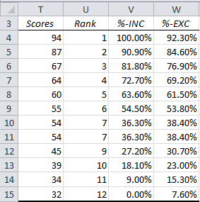
Example 9: Repeat Example 5 using the PERCENTRANK.INC and PERCENTRANK.EXC functions.

The result is shown in Figure 7. E.g. the score 45 (cell T12) is at the 27.2^th percentile (cell V12) using the formula =PERCENTRANK.INC(T4:T15,T12), while it is at the 30.7^th percentile (cell W12) using the formula =PERCENTRANK.EXC(T4:T15,T12).

Figure 7 – PERCENTRANK vs. PERCENTRANK.EXC

QUARTILE

Definition 6: For any integer k = 0, 1, 2, 3, or 4, QUARTILE(R1, k) = PERCENTILE(R1, k/4). If c is not an integer, but 0 ≤ c ≤ 4, then QUARTILE(R1, c) = QUARTILE(R1, INT(c)).

Observation:

• QUARTILE(R1, 0) = PERCENTILE(R1, 0) = MIN(R1)
• QUARTILE(R1, 1) = PERCENTILE(R1, .25)
• QUARTILE(R1, 2) = PERCENTILE(R1, .5) = MEDIAN(R1)
• QUARTILE(R1, 3) = PERCENTILE(R1, .75)
• QUARTILE(R1, 4) = PERCENTILE(R1, 1) = MAX(R1)

Example 10: For range R1 with data elements {4, 0, -1, 7, 5}

• QUARTILE(R1, 0) = PERCENTILE(R1, 0) = -1
• QUARTILE(R1, 1) = PERCENTILE(R1, .25) = 0
• QUARTILE(R1, 2) = PERCENTILE(R1, .5) = 4
• QUARTILE(R1, 3) = PERCENTILE(R1, .75) = 5
• QUARTILE(R1, 4) = PERCENTILE(R1, 1) = 7

Excel Worksheet Functions

Releases of Excel after Excel 2007 provide two versions of the quartile function: QUARTILE.INC and QUARTILE.EXC. The first of these is equivalent to QUARTILE and the second is defined so that QUARTILE.EXC(R1,  k) = PERCENTILE.EXC(R1,  k/4).

Real Statistics Function

The Real Statistics Resource Pack provides the following worksheet function.

QUARTILE_EXC(R1, k, m) = PERCENTILE_EXC(R,  k/4, m)

m takes integer values between 1 and 8 (as for PERCENTILE_EXC). If omitted, m defaults to 6. Thus QUARTILE_EXC(R1, k) = QUARTILE.EXC(R1, k) for k = 1, 2 or 3, but QUARTILE_EXC(R1, 0) = MIN(R1) and QUARTILE_EXC(R1,4) = MAX(R1) instead of outputting an error value.

Examples Workbook

Click here to download the Excel workbook with the examples described on this webpage.

References

Hyndman, R. J., Fan, Y. (1996) Sample quantiles in statistical packages
https://www.amherst.edu/media/view/129116/original/Sample+Quantiles.pdf

Calder, S. (2023) How to calculate percentile in Excel?
https://www.simonsezit.com/article/calculate-percentile-in-excel/