We now consider the case where the two sample pairs are not drawn independently because the two correlations have one variable in common.
Click here for the case where the sample pairs don’t overlap.
Click here for the case where the sample pairs are independent.
Example
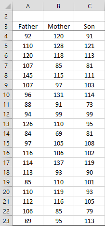
Example 1: IQ tests are given to 20 couples. The oldest son of each couple is also given an IQ test with the scores displayed in Figure 1. We would like to know whether the correlation between son and mother is significantly different from the correlation between son and father.
Figure 1 – Data for Example 1
We will use the following test statistic
where S is the 3 × 3 sample correlation matrix (see Multiple Correlation for details) and
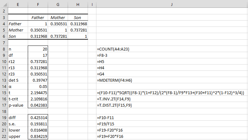
(see Determinant). For this problem, the results are displayed in Figure 2, where the upper part of the figure contains the correlation matrix S (e.g. the correlation between Mother and Son is calculated by the function =CORREL(B4:B23,C4:C23) and is shown in cells H5 and G6).
The 95% confidence interval is calculated in the usual way using the fact that the standard error is the reciprocal of the square root term in the definition of t.
Figure 2 – Analysis for Example 1
Since p-value = .042 < .05 = α (or t < t-crit) we reject the null hypothesis and conclude that the correlation between mother and son is significantly different from the correlation between father and son.
Worksheet Functions
Real Statistics Functions: The following array functions are provided in the Real Statistics Resource Pack.
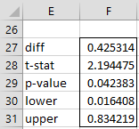
Correl2OverlapTTest(r12, r13, r23, n, alpha, lab): array function which outputs the difference between the correlation coefficients r12 and r13, t statistic, p-value (two-tailed) and the lower and upper bounds of the 1 – alpha confidence interval, where r12 is the correlation coefficient between the first and second samples, r13 is the correlation coefficient between the first and third samples, r23 is the correlation coefficient between the second and third samples and n is the size of each of the three samples.
If lab = TRUE then the output takes the form of a 5 × 2 range with the first column consisting of labels, while if lab = FALSE (default) then the output takes the form of a 5 × 1 range without labels; if alpha is omitted it defaults to .05.
Corr2OverlapTTest(R1, R2, R3, alpha, lab) performs the two sample correlation test for samples R1, R2 and R3 where R2 is the overlapping sample. This array function return the array from =Correl2OverlapTTest(r12, r13, r23, n, alpha, lab) where r12 = CORREL(R1, R2), r13 = CORREL(R1, R3), r23 = CORREL(R2, R3) and n = the common sample size for R1, R2 and R3.
For Example 1, the output from =Correl2OverlapTTest(F6,G6,G4,F8,,TRUE) is shown in Figure 3. 
Figure 3 – Test using Real Statistics function
The same output is produced by the function
=Corr2OverlapTTest(C4:C23,A4:A23,B4:B23,,TRUE)
Fisher Approach
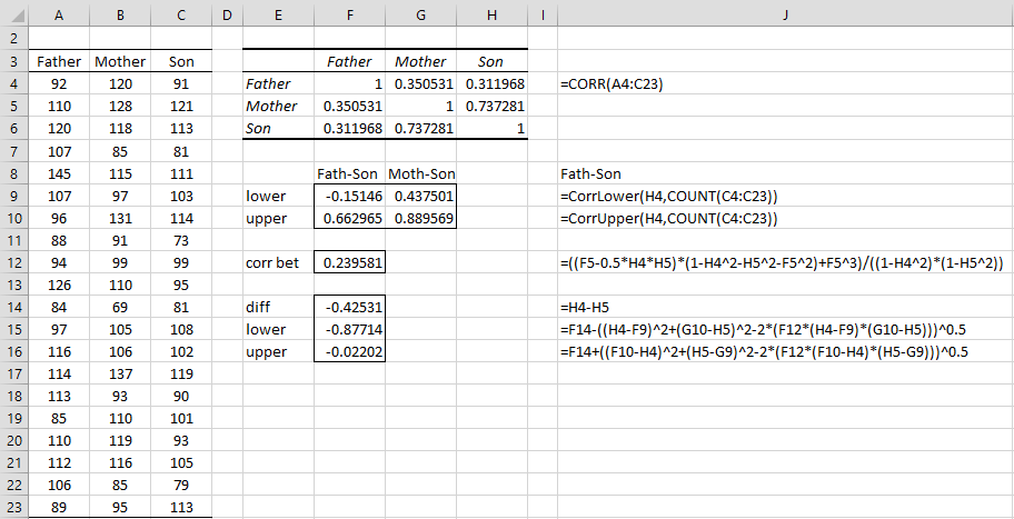
We can perform another version of this two-sample correlation test using the Fisher transformation, as shown in Figure 4.
Figure 4 – Fisher analysis for Example 1
As you can see from range F15:F16, the 95% confidence interval calculated this time (taking absolute values) is (02202, .87714). This is not so different from the interval calculated in Figure 2, namely (016408, .834219).
Worksheet Functions (Fisher approach)
Real Statistics Functions: The following array functions are provided in the Real Statistics Resource Pack to implement the Fisher test described above.
Correl2OverlapTest(r12, r13, r23, n, alpha, lab)
Corr2OverlapTest(R1, R2, R3, alpha, lab)
These functions are identical to Correl2OverlapTTest(r12, r13, r23, n, alpha, lab) and Corr2OverlapTTest(R1, R3, R2, alpha, lab) except that the Fisher transformation is used as described above and the output only has three elements: the difference between the correlations and the endpoints of the confidence interval.
For Example 1, the output from =Correl2OverlapTest(F6,G6,G4,F8,,TRUE) is as shown in range F14:F16 of Figure 3. The same output is produced by the array function
=Corr2OverlapTest(C4:C23,A4:A23,B4:B23,,TRUE)
Examples Workbook
Click here to download the Excel workbook with the examples described on this webpage.
References
Howell, D. C. (2010) Statistical methods for psychology (7th ed.). Wadsworth, Cengage Learning.
https://labs.la.utexas.edu/gilden/files/2016/05/Statistics-Text.pdf
Rousselet, G. A. (2017) How to compare dependent correlations
https://garstats.wordpress.com/2017/03/01/comp2dcorr/


Dear Charles,
Is it possible to test a hypothesis like r1-r2/r3>0 or r1*r3-r2>0, where r1,r2,and r3 are pair-wise correlation coefficients with overlapping variables? I am struggling to find the test-statistics for this case.
Thank you.
Ratbek
Dear Ratbek,
I am not sure why you would want to test r1*r3>r2, but, in any case, I don’t know a method for testing this.
Charles
Why is that the UDFs, Corr2OverlapTTest and Corr2OverlapTest, return the same Difference values but with opposite signs? That is, 0.425313556 and -0.425313556? Even the CI with Corr2OverlapTest is negative.
If I remember correctly, the sign is unimportant in this case.
Charles
Good Morning Prof. Zaiontz,
first of all, thank you for this detailed page!
I’ve got a problem, on which I’m spinning my head around, and therefor a tricky question for you:
I have two datasets (patients and age/sex matched controls, but different N) with n repeated measures (basically it’s some derived MRI scores in ascending coordinates). Since some assumptions for an rmANOVA are not met and transformation doesn’t help, I’m searching for other ways to examine the interaction.
I assume a priori a linear dependency of my DV on the the n measurements, so I got the idea of just comparing the correlations. But now I’m a bit stuck in the decision on how to do so exactly.
My first impulse was to average the DV per n in each cohort, then compute the correlations etc. as suggested above (I suppose it’s William’s t). Here, I get a significant difference for r(data1, n) and r(data2, n).
But supposing that the groups are independent, I’d rather go with the method suggested in ‘Two Sample Hypothesis Testing for Correlation’ (which is Fishers z’). Here, I computed the correlations r(DV, n) per subject, transformed them into z and averaged them, and eventually inverted them back to rs. Thus, I input two mean correlations mr(data1, n), mr(data2, n) with the corresponding Ns in the comparison. This outputs no significant difference.
So, which one’s the correct method to apply?! I’m at a point where my thoughts drive in a roundabout, so I hope you can bring some light in this mess and maybe give me a hint, I would really appreciate it. 🙂
Kind regards from Germany
Martin
Martin,
Let me make sure I understand the basics of the situation. From what I see, you have the follow situation.
Data set 1 (treatment): N1 elements and n repeated measures (not replication!). E.g. 20 patients with a blood pressure reading at 9am, 12pm, 3pm, 6pm. Here N1 = 20 and n = 4
Data set 2 (control): N2 elements and n repeated measures, where N1 and N2 may be different
Please let me know whether this is correct. Also what hypothesis are you trying to test? I would prefer an answer in experimental terms and not statistical terms.
Charles
Charles,
thank you for your quick answer.
Your basic assumption is right, only that precisely it’s N1=73, N2=59 and n is 16 (41 respectively). n represents brain coordinates and the DV is an average MRI score. The basic question of my research is, whether there is a significant group difference of the DV’s dependency on the coordinate. The presumption is, that the dependency is linear, so Pearson’s r is indicated. Therefor, I could examine the difference in the gradient/slope of the linear fit.
Best,
Martin
You haven’t provided any way to pair the values in group 1 with those in group 2, and so I don’t see how to calculate r. If n1 : n2, we could compare the groups to see whether they have the same means, but since n1 is not equal to n2, I don’t see how to do that either.
Charles
Ah, sorry for the misunderstanding: n is equal for both groups! I just have 2 different comparisons one time n is 16, another time it’s 41, but always the same for both groups. Sorry, admittedly my expression was misleading!
Can I get the proof for this formula? Thanks a lot.
Richard,
I don’t have the proof of either approach. I discovered the first approach (presumably the one you are referencing) in David Howell’s textbook. He is referencing a paper by Williams, E.J. (1959). See Bibliography for details.
Charles
Good Nigt mr.charles, i want to ask you about the simbol of ~T(n-3), what does it mean? especially the T simbol. Thank you.
from Indonesia 🙂
x ~ T(n-3) means that the random variable x has a t distribution with n-3 degrees of freedom. It can also mean that x has approxomately a t distribution with n-3 degrees of freedom.
Charles
If I understand it correct this is versus the alternative that their IQ:s are different.
Now if I want to make a one sided test of this, should go about the same way as in previous examples?
Gustaf,
This is a one sided test.
Charles
Dear Professor Zaiontz,
I am a medical student persueing master degree from China. I am really greatful for your sharing this wonderful formula with us on the web, for I want to take this statistic into my writing article. But I wonder where this formula comes from. Would you please tell me the references? Thanks a lot.
My best wishes.
Yoyo Gong
The reference is Howell, D. C. (2010). Statistical methods for psychology (7th ed.). Wadsworth, Cengage Learning.
Charles
Thanks a lot. This is quite useful for me.