Polychoric Correlation Basic Concepts

Introduction

When data is organized in the form of a contingency table (see Independence Testing) where the two categorical independent variables (corresponding to the row and columns) are ordered, then we can calculate a polychoric correlation coefficient. This coefficient is an approximation to what Pearson’s correlation coefficient would be if we had continuous data. For a 2 × 2 contingency table, the polychoric correlation coefficient is called the tetrachoric correlation coefficient.

You can think of the tetrachoric correlation between two dichotomous variables x and y as Pearson’s correlation between x′ and y′ where x′ and y′ are “latent” variables that are normally distributed (actually bivariate normally distributed) and x = 1 when x′ > c and y′ = 1 when y′ > d for some unknown constants c and d.

Example

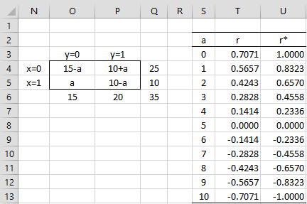
Looking at the marginal totals on the left side of Figure 1, we see that cell O5 can take any integer value between 0 and 10. Pearson’s correlation coefficient for each of these options is shown in column T. Cell T3, for example, contains the formula =SQRT(CHI_STAT(O4:P5)/Q6) where 0 is inserted in cell O5, and similarly for the other cells in column T (see Chi-square Effect Size). Note that the values range from -.7071 to .7071.

The corresponding tetrachoric correlation coefficients shown in column U are higher than the corresponding Pearson’s correlation coefficients and range from -1 to +1. In Tetrachoric Correlation Estimation we show how to calculate these tetrachoric correlation coefficients (using method 1 estimates).

Figure 1 – Comparing Pearson’s and tetrachoric correlation

Example Resolution

For example, suppose we have a 2 × 2 with the marginal totals shown in Figure 1.

The situation is similar for the polychoric correlations. Suppose we have an m × n contingency table. In this case, x can take values 0 to m–1 and y can take values 0 to n–1. We now have constants c₀, …, c_m and d₀, …, d_n where c₀ = d₀ = -∞ and c_m = d_n = ∞ and latent variables x′ and y′ such that x = i when c_i < x′ ≤ c_i+1 and y = j when d_j < y′ ≤ d_j+1.

If x ∼ N(μ, σ²), then P(x = i) = NORM.DIST(c_i+1, μ, σ, TRUE) – NORM.DIST(c_i, μ, σ, TRUE). In fact, if we set u_i = (c_i – μ)/σ, then P(x = i) = NORM.S.DIST(u_i+1, TRUE) – NORM.S.DIST(u_i, TRUE), which is the area under the standard normal curve between x = u_i+1 and x = u_i. The same is true for y′. Henceforth, we will assume that we are using standard normal distributions and use the constants c_i instead of u_i, and similarly for d_j.

Suppose that the elements in the contingency table are h_ij. Then the marginal total for the i^th row in the contingency table is a_i = h_ij and the marginal total for the j^th row is b_j = h_ij, with a grand total of g =  a_i =  b_j.

A natural estimate for c_i for 0 < i < m is c_i = NORM.S.INV(a_i/g) and a natural estimate for d_j for 0 < j < n is d_j = NORM.S.INV(b_j/g).

Now, assuming bivariate normality, we also have

P(x = i, y = j) = BNORMSDIST(c_i+1,d_j+1,ρ,TRUE) – BNORMSDIST(c_i+1,d_j,ρ,TRUE)

where BNORMSDIST(x, y, ρ, TRUE) is the Real Statistics formula that computes the bivariate standard normal distribution (cdf) at (x, y) when the correlation coefficient is ρ (see Multivariate Normality Functions).

Note, however, that BNORMSDIST(x, y, ρ, TRUE) is not defined when x or y is equal to ±∞. In these cases, we consider

BNORMSDIST(–∞, y, ρ, TRUE) = BNORMSDIST(x, ∞, ρ, TRUE) = 0

BNORMSDIST(∞, y, ρ, TRUE) = NORM.S.DIST(y, TRUE)

BNORMSDIST(x, ∞, ρ, TRUE) = NORM.S.DIST(x, TRUE)

BNORMSDIST(∞, ∞, ρ, TRUE) = 1

Examples Workbook

Click here to download the Excel workbook with the examples described on this webpage.

References

Uebersax, J. S. (2015) Introduction to the tetrachoric and polychoric correlation coefficients
http://www.john-uebersax.com/stat/tetra.htm

Mahler, C.M. (2016) The tetrachoric correlation coefficient
https://eigenblogger.com/tag/tetrachoric-correlation-coefficient/

STATA (2017) Tetrachoric correlations for binary variables
www.stata.com/manuals13/rtetrachoric.pdf