Basic Concepts
The lambda coefficient is a measure of (asymmetric) association that reflects the proportional reduction in error (PRE) when values of the independent variable are used to predict values of the dependent variable. Lambda takes values between 0 and 1. A value of 1 means that the independent variable perfectly predicts the dependent variable. A value of 0 means that the independent variable is no help in predicting the dependent variable.
We assume that we have a contingency table where the rows R represent the independent variable and the columns C represent the dependent variable. We show how to calculate λ(C|R).
Example
Example 1: The contingency table in Figure 1 displays the frequency with which a sample of 400 teenagers in 8 neighborhoods (A-H) express a preference for hamburger, pizza, or panino. Which food would you predict teenagers prefer and what is the probability that you would guess this preference correctly? What is the improvement in the prediction if you also know the neighborhood of the teenager?
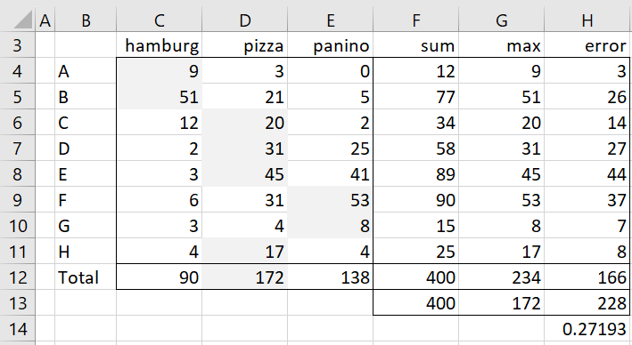
Figure 1 – Food preference by neighborhood
With only the aggregate information, shown in row 12, we see that pizza is the food preferred by teenagers in the sample, and so if you had to predict what any teenager would prefer, then pizza would be your best guess. You would be right 172/400 = 43% of the time and wrong 228/400 = 57% of the time. Here 228 and 57% represent the error in the prediction.
Now if you had additional information about the teenager’s neighborhood, you could improve your prediction by 27% (cell H14). E.g. if you knew that the teenager came from neighborhood A, from the contingency table you see that your best prediction is hamburger since the is the food preferred in that neighborhood. The error in the prediction for this neighborhood is 3 (cell H4). If for each neighborhood you choose the food preference for that neighborhood (as highlighted in Figure 1), you would have a total error of 166.
The reduction in error is therefore equal to 1-166/228 = 27.2% (cell H14). This is the value of lambda, and it represents the improvement in the prediction by having the additional information represented by the independent variable (neighborhood in this example). In fact, lambda can also be calculated as (234-172)/(400-172) = 62/228 = .27193.
Lambda(C|R) Formulas
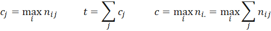
In general, we can calculate lambda by
![]()
Here nij = the frequency value in the ith row and jth column and

Thus, n = the sum of all the frequencies in the contingency table. For each row i, ri = the largest element in that row. s = the sum of all the ri and r = the largest column total in the contingency table.
Hypothesis Testing
The standard error of the lambda coefficient is
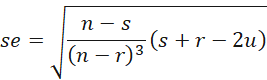
where
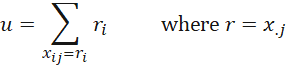
Thus, u is the sum of the ri that occur in the jth column where j is the column where the maximum value of the column sums occurs. For Example 1, j = 2, and u = 20+31+45+17 = 113. Note that if more than one column such that r = x.j then choose the leftmost column. (Actually, u may be overstated when in any row i, multiple cell values = ri, but we will ignore this).
Confidence Interval
The 1-α confidence interval is
λ ± se ⋅ zcrit
where zcrit = NORM.S.DIST(-ABS(α/2),TRUE).
We see from Figure 2 that lambda is significantly different from 0 (p-value << .05). The 95% confidence interval for lambda in Example 1 is (.1735, .3703) as shown in cells K15 and K16. Thus, there is a significant asymmetric association between the two variables, and knowing the neighborhood improves the prediction of a teenager’s preferred food.
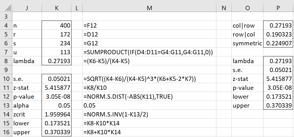
Figure 2 – Testing and Confidence interval
Lambda(R|C)
Note that we get a different value for lambda, namely λ(R|C), if we assume that the columns represent the independent variable, and the rows represent the dependent variable. For this reason, we call lambda a measure of asymmetric association. In fact,
![]()
where
For Example 1,
![]()
Symmetric Lambda
We also have a symmetric version of lambda, defined as
![]()
For Example 1,
![]()
Worksheet Functions
Real Statistics Functions: The Real Statistics Resource Pack provides the following function for R1 that contains a contingency table (w/o headings or totals).
LAMBDA_COEFF(R1, lab): returns a column array with lambda(C|R), lambda(R|C), and symmetric lambda for the data in R1.
LAMBDA_TEST(R1, lab, alpha, lambda0): returns a column array with lambda(C|R), standard error, z-stat, p-value, and lower and upper ends of the 1-alpha confidence interval.
If lab = TRUE (default FALSE) then an extra column of labels is appended to the output. alpha is the significance level (default .05). The z-statistic is equal to (lambda – lambda0)/s.e. If lambda0 is omitted, it defaults to zero. Note that the confidence interval is based on lambda0 = 0 even when lambda0 is specified.
For Example 1, the formula =LAMBDA_TEST(C4:E11,TRUE) produces the output shown in range O8:P13 of Figure 2.
For the data in Example 1, the formula =LAMBDA_COEFF(C4:E11,TRUE) produces the output shown in range O4:P6 of Figure 2.
Data Analysis Tool
Real Statistics Data Analysis Tool: The Real Statistics Resource Pack provides the Association Tests data analysis tool that can be used to calculate the lambda statistic and can be used to test whether λ = λ0.
For Example 1, you need to press Ctrl-m and select Association Tests from the Corr tab. Next, fill in the dialog box that appears as shown in Figure 3.
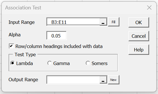
Figure 3 – Association Tests dialog box
After clicking on the New button (next to the Output Range field) and clicking on the OK button, the output shown on the left side of Figure 4 appears.
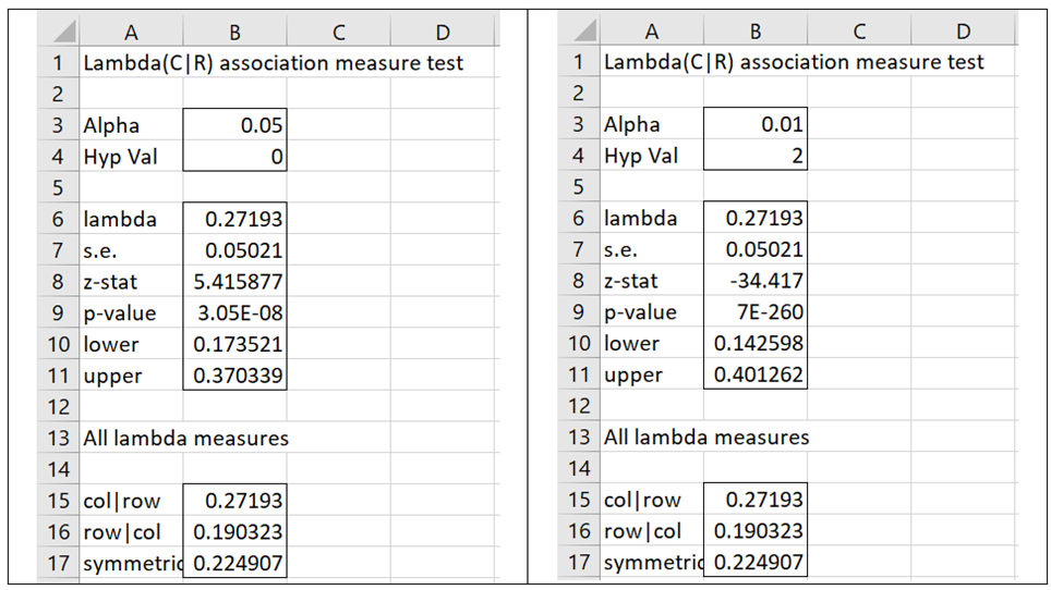
Figure 4 – Association Tests output for Lambda
Suppose that you want to test the null hypothesis λ = 2 at the α = .01 significance level. You can then change the value in B3 to .01 and the value in B4 to 2. The result is shown on the right side of Figure 4.
Examples Workbook
Click here to download the Excel workbook with the examples described on this webpage.
References
SAS (2018) The frequency procedure. User’s guide
https://support.sas.com/documentation/onlinedoc/stat/151/freq.pdf
Holbrook, T. M. (2022) Measures of association. An introduction to political and social data analysis using R
https://collegepublishing.sagepub.com/products/an-introduction-to-political-and-social-data-analysis-with-r-1-288105
Bonett, D. (2014) Asymptotic standard error of lambda
https://lists.gnu.org/archive/html/pspp-dev/2014-05/msg00007.html