Fundamental Property
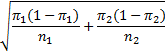
Property 1: Let x1 and x2 be two random variables that have a proportion distribution with means π1 and π2 respectively. Let p1 be the proportion of successes in n1 trials of the first distribution and let p2 be the proportion of successes in n2 trials of the second distribution. When the number of trials n1 and n2 is sufficiently large, usually when ni πi ≥ 5 and ni (1 – πi) ≥ 5, the difference between the sample proportions p1 – p2 will be approximately normally distributed with mean π1 – π2 and standard deviation
Proof: Based on Property 2 of the Binomial Distribution, xi has approximately the distribution N(πi, πi(1–πi)/ni).
Since x1 and x2 are independently distributed, by the linear transformation property of the normal distribution (Properties 1 and 2 of Normal Distribution), x1–x2 has a normal distribution with mean π1–π2 and a standard deviation that is the square root of π1(1–π1)/n1+π2(1–π2)/n2.
Example
Example 1: A company that manufactures long-lasting light bulbs sells halogen and compact fluorescent bulbs. They conducted an experiment in which they ran 100 halogen and 100 fluorescent bulbs continuously for 250 days. They found that half of the halogen bulbs were still working while 60% of the fluorescent bulbs were still operating. Is there a significant difference between the two types of bulbs?
Let x1 = the percentage of halogen bulbs that are functional after 250 days and x2 = the percentage of fluorescent bulbs that are functional after 250 days. The presumption is that the distributions for each of these are proportional. We now test the following null hypothesis:
H0: π1 = π2
Assuming the null hypothesis is true, by Property 1, x1 – x2 will be approximately normal with mean π1 – π2 = 0 and standard deviation
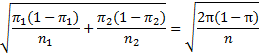
where the common value of the mean is denoted π and both samples are of size n. Since the value for π is unknown, we estimate its value from the sample, namely, 50 + 60 = 110 successes out of 200 trials, i.e. π ≈ 0.55, Thus, the mean of x1 – x2 is 0 (based on the null hypothesis) and the standard deviation is approximately (.45)}{100}}")
p-value = NORM.DIST(.1, 0, .704, TRUE) = .922 < .975 = 1 – α/2
Thus, we can’t reject the null hypothesis and so we cannot conclude there is a significant difference between the two types of bulbs.
Alternative Approaches
We reach the same conclusion via either of the following tests:
p-value = 2*(1–NORM.DIST(.1, 0, .0703, TRUE)) = .155 > .05 = α:
critical value of x1 – x2 = NORM.INV(.975,0,.0703) = .138 > .1 = observed value of x1 – x2
Examples Workbook
Click here to download the Excel workbook with the examples described on this webpage.
References
Stat Trek (2021) Hypothesis test: difference between two proportions
https://stattrek.com/hypothesis-test/difference-in-proportions.aspx
Shafer and Zhang (2021) Comparison of two population proportions. Introductory Statistics
https://stats.libretexts.org/Bookshelves/Introductory_Statistics/Book%3A_Introductory_Statistics_(Shafer_and_Zhang)/09%3A_Two-Sample_Problems/9.04%3A_Comparison_of_Two_Population_Proportions
Thank you so much again for your wonderful site. Not only am I able to do complex analyses which are very informative, but I am learning a great deal. I have a question about whether I can use two sample proportion testing for the following situation.
I am looking at causes of death in a particular population. The population consists of 209 individuals who had some college education and 109 individuals who had none. 13 of the people in the first population died of accidental causes. 20 of the people in the second population died of accidental causes. In other words, the proportion of people in the second population dying of accidents was more than double that of the first population. Using the two sample proportions application from your website, it would seem that this difference is significant. However, I am not sure whether I am using the two sample proportion test correctly because my application is very different from other ones on the site. Thanks again.
Hi Ruth,
I am pleased that you are getting value from the website. Glad I could help.
It seems like you are using the right approach. Your example is similar to the example described on the webpage, except that the sample sizes are different for your analysis.
Charles
That is terrific Charles, thanks so much again. Because of your site, I can see very clearly what the data are saying.
Might I ask another question. I love the ability to do contrasts after Welch’s ANOVA or Kruskal-Wallis. I am comparing individuals with no college, individuals with at least some college, and individuals with higher education. One example of the type of thing I am looking at is income. I want to compare the middle group (some college) to each of the other two groups. My understanding is that this would be 2 comparisons, so that is what I entered when I did the initial analysis.
On the chart of comparisons, should I fill in 1 for the middle group (some college) and -0.5 for each of the other two groups? I am unclear as to whether this is only comparing the middle group to each of the others, or whether the two others are also being compared. In addition, the middle group is not the highest in income, and the +1 should be for this highest, as I understand it.
Alternately I could fill in the contrasts table twice. First for no college (-1) and some college (+1), and then for some college (-1) and graduate education (+1).
Thanks so much for any advice you might have.
Ruth,
It really depends on what hypothesis you want to test.
If you want to compare the middle group with the average of the other two groups, then you should use +1 for the middle group and -.5 for the other two groups. Whatever you do, the sum of the contrast weights must be 0. This is considered to be one comparison. You don’t need to use +1 for the highest.
If instead, you want to compare the middle group with each of the other two groups, you would perform 2 comparisons. The first would use +1 for middle and -1 for highest (or -1 for middle and +1 for highest, which would result in a positive difference instead of a negative difference) and a second comparison where you used +1 for the middle group and -1 for the smallest group. Note that you need to decide in advance which contrast comparisons you want to test.
If you plan to restrict yourself to pairwise comparisons, then you should consider using Tukey’s HSD test instead of contrasts.
Charles
This is very helpful Charles. I want to compare the middle group (some college) to each of the other two groups (no college, graduate school). Therefore I will do 2 comparisons, +1 and -1.
I like the idea of using Tukey’s HSD. One thing is that my group sizes are very different. The output numbers do not really follow a normal distribution very well (often shifted to the right). For one of the comparisons I want to make of the three groups, one groups is not symmetric. For another comparison, the variances of the three groups range from about 100 to 200.
All in all, I am not sure which test to use.
I used multiple regression on the data set as a whole. I found that the upper and lower groups differed from the middle group . However, it is not clear to me whether this means the the upper and lower differed from the middle group on each component of the regression (e.g., it is not clear whether they specifically differ in terms of income).
Again, thank you so much for your help. I hope this this explanation is fairly clear.
Hi Ruth,
Even when the variance of one group is 2 times the other, these tests usually give pretty good results.
The Tukey-Kramer post-hoc test handles the case where the group sample sizes are quite different. Fortunately, the Real Statistics implementation of the Tukey HSD test automatically yields the Tukey-Kramer test when the group sizes are different (the Tukey HSD test is just a special case of Tukey-Kramer).
If the variances are really quite different, then you can use the Graham-Howell post-hoc test instead of Tukey HSD.
All these tests are pretty robust to violations of normality, but if there is doubt, you can use one of the nonparametric tests.
I am not sure how you used multiple regression to identify differences between the groups, but keep in mind that behind-the-scenes ANOVA is really multiple regression, and so the ANOVA results are really regression results.
Charles
ok, that is very good information Charles about the Tukey HSD and Tukey Kramer. Also about multiple regression and ANOVA.
In some ways, I would love to do a nested ANOVA. The reason relates to the fact that I have these three major groups, but they can be broken down into subgroups. The upper and lower education groups definitely exhibit differences from the middle group. However, if I analyze the subgroups, well I have rather small numbers of people in the subgroups.
Will look into Tukey. Much appreciate your advice and expertise.
Hi Dr Zaiontz,
I am trying to solve this problem:
I am going to perform 2 samples with equal number of trials each (n1=n2). From each sample I will obtain p1 and p2, which estimate the real probabilities prob1 and prob2 of the 2 populations.
I want to figure out for a certain range of delta=p1-p2 (say 0.1 to 0.5) what sample size I require to refute H0: p1=p2 with alpha=o.o5, 2 tails and power=80%.
Also, when I choose an appropriate sample size, I would like to plot the power of the two sample test against delta=p1-p2.
Which example is closest to answering my question and which excel function do you suggest?
Thank you
Ivan
Ivan,
You can use the Proportions option of the G*Power power/sample size tool. You can download it free from https://g-power.apponic.com/.
I also plan to add this to Real Statistics in a future release.
Charles
Dr. Zainonitz good nights, since in Spanish excel the normal distribution goes from less infinity to more infinity, the formula would not have an absolute value?
= 1-STANDARD NORMDIST (ABS ((D23-E23)) / ROOT (D23 * (1-E23) / F22 + E23 * (1-E23) / F22))
Thank you very much
Hello Gerardo,
Nice to hear from you again.
Are you asking whether (1) your formula is correct or are you suggesting that (2) the formula listed on the webpage is not correct or (3) both?
Charles
Doc, good afternoon, thank you very much, excuse me for being late in replying. I am suggesting to make the change, because there is an error in the Spanish excel.
Gerardo,
I presume that the formula you are referring to is
= 1-NORMSDIST(ABS(D23-E23)/SQRT(D23*(1-E23)/F22+E23*(1-E23)/F22)) or
= 1-NORM.S.DIST(ABS(D23-E23)/SQRT(D23*(1-E23)/F22+E23*(1-E23)/F22),TRUE)
I don’t see such a formula on the webpage or in the examples workbook. Please explain further what the problem is with this formula.
Charles
Please excuseme, because i am late, Yes Sr, exactly
= 1-NORMSDIST(ABS(D23-E23)/SQRT(D23*(1-E23)/F22+E23*(1-E23)/F22))
Thanks
Dear Gerardo,
My apologies for such a late reply.
If I understand correctly, the formula = 1-NORMSDIST(ABS(D23-E23)/SQRT(D23*(1-E23)/F22+E23*(1-E23)/F22)) produces an error when used in the Spanish version. Can you tell me (1) where this formula is being used and (2) what sort of error occurs in the Spanish version?
My apologies if you have answered one or both of these questions previously.
Charles