One-sample Proportion Testing

Basic Approach

From Property 1 of Proportion Testing Basic Concepts, we know that when samples of size n are drawn, for n sufficiently large, the distribution of sample proportions is approximately normal, distributed around the true population proportion mean π, with standard deviation (i.e. standard error) of

We can use this fact to do hypothesis testing as was done for the normal distribution. In addition, when a two-tailed test is performed a confidence interval can be calculated where

If necessary, we can use the sample mean p as an estimate for the population mean when calculating the standard error. This introduces an additional error, which is acceptable for large values of n.

Two-tailed Test

Example 1: A company believes that 50% of its customers are women. A sample of 600 customers is chosen and 325 of them are women. Is this significantly different from their belief?

H₀: π = 0.5; i.e. any difference in the number of men and women is due to chance
H₁: π ≠ 0.5

Method 1: Using the binomial distribution, we reject the null hypothesis since:

BINOM.DIST(325, 600, .5, TRUE) =  0.981376 > 0.975 = 1 – α/2 (2-tailed test)

Method 2: By Property 1 of Relationship between Binomial and Normal Distributions, we can use the normal distribution as follows.

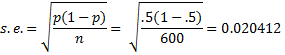
The observed mean is 325/600 = 0.541667. Based on the null hypothesis, we can assume that the mean is p = .5 and the standard error is

Now

NORM.DIST(.541667, .5, .020412, TRUE) = 0.979387 > 0.975 = 1 – α/2 (2-tailed)

and so we reach the same conclusion, namely to reject the null hypothesis.

One-tailed Test

Example 2: A survey of 1,100 voters showed that 53% are in favor of the new tax reform. Can we conclude that the majority of voters (from the population) are in favor?

We use the following (one-tailed) null hypothesis:

H₀: π ≤ 0.5

Since people are not surveyed twice, we essentially have a hypergeometric distribution instead of a binomial distribution; i.e. we are selecting without replacement. But for large n the hypergeometric distribution is approximately binomial (i.e. it is not so likely that you will select the same person twice).

Since p = .53 and n = 1100, it follows that np ≥ 5 and n (1 – p) ≥ 5. Thus, we can approximate the distribution by a normal distribution. Using p as an estimate for π in calculating the standard error, we obtain

Since NORM.DIST(.53, .5, 0.01505, TRUE) = .976889 > .95, we reject the null hypothesis and conclude with 95% confidence that the population will vote in favor of the tax reform.

Confidence Interval

Based on a two-tailed test, we can determine the 95% confidence interval for Example 2 as follows:

z_crit = NORM.S.INV(1 – α/2) = NORM.S.INV(0.975) = 1.96

and so the 95% confidence interval is

p ± z_crit ⋅ s.e. = .53 ± 1.96 ⋅ 0.01505 = .53 ± 0.029

We conclude with 95% confidence that between 50.1% and 55.9% of the population will be in favor of the tax reform. If instead, we are looking for a 99% confidence interval, the calculation would be:

 z_crit = NORM.S.INV(1 – α/2) = NORM.S.INV(0.995) = 2.58

and so the 99% confidence interval is

p ± z_crit ⋅ s.e. = .53 ± 2.58 ⋅ 0.01505 = .53 ± 0.039

This is a confidence interval of (49.1%, 56.9%). Since 50.0% is in this interval, this time we cannot conclude with 99% confidence that the population will vote in favor of the tax reform.

Sample Size Example

Example 3: In conducting a survey of potential voters, how big does the sample need to be so that with 95% confidence the actual result (i.e. the population mean) will be within 2.5% of the sample mean? (i.e. how big a sample is necessary to have a 2.5% margin of error?)

This time we are looking for the value of n such that

z_crit · s.e. = 2.5%

As we saw in the previous example for 95% confidence z_crit = 1.96. We now need to determine when the standard error is at its the maximum (for any specific value of n). For any n, s.e. = is maximum when p(1–p) is maximum. It is not hard to see that this occurs when p = .5. Thus the maximum s.e. = = . It now follows that

Solving for n yields n = 1536.584. Thus a sample of size 1,537 is sufficient. Using a similar calculation, achieving a 99% confidence requires a sample size of 2,654.

Examples Workbook

Click here to download the Excel workbook with the examples described on this webpage.

References

Kozak, K. (2021) One-sample proportion test. Statistics using technology
https://stats.libretexts.org/Bookshelves/Introductory_Statistics/Book%3A_Statistics_Using_Technology_(Kozak)/07%3A_One-Sample_Inference/7.02%3A_One-Sample_Proportion_Test

Boston University School of Public Health (2016) One sample test of proportions
https://stats.libretexts.org/Bookshelves/Introductory_Statistics/Statistics_with_Technology_2e_(Kozak)/07%3A_One-Sample_Inference/7.02%3A_One-Sample_Proportion_Test