We now provide some examples of how to use the geometric distribution, which is a special case of the negative binomial distribution.
Example
Example 1: The probability that Bob hits a free throw in basketball is 20%. He decides to continue to attempt free throws until he makes one of them. What is the probability that he will miss five times before making one? What is the probability that he will miss at most five times before making one?
The probability that he will miss five times before making one is 6.55% (cell B6 of Figure 1). The probability that he will miss at most five times before making one is 73.8% (cell B7).
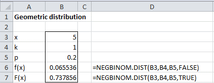
Figure 1 – Example of geometric distribution
Since the cdf is not supported in versions of Excel prior to Excel 2010, Excel 2007 users need to use the approach shown in Figure 2.
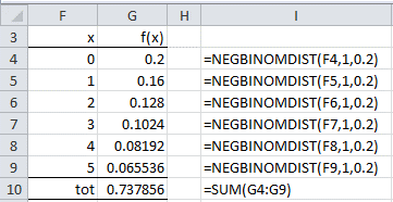
Figure 2 – Example of geometric distribution in Excel 2007
Excel Trick
The following Excel 2007 worksheet formula is equivalent to =NEGBINOM.DIST(5,1,.2,TRUE)
=SUMPRODUCT(NEGBINOMDIST(ROW(INDIRECT(“1:6”))-1,1,0.2))
and so has the value 0.737856. This formula works since the INDIRECT array function takes a string with a cell or range address and outputs the reference address. E.g. =INDIRECT(“A1:A10”) outputs the range A1:A10 and the array formula =ROW(INDIRECT(“1:6”)) outputs a column range containing the values 1, 2, 3, 4, 5, 6. We could replace SUMPRODUCT with SUM in the above formula, but then we would have to press Ctrl-Shft-Enter instead of just Enter.
Similarly, we can put the following formula in cell B7 of Figure 2:
=SUMPRODUCT(NEGBINOMDIST(ROW(INDIRECT(“1:”&B3+1))-1,B4,B5))
Another Example
Example 2: What is the average number of tosses of one die required to obtain all six possible values? What is the standard deviation?
Let x = the number of tosses required to obtain all six values.
We used simulation to create an estimate of the mean and standard deviation of x in Simulating a Distribution. We will now use the geometric distribution to obtain an exact value.
Let xi be a random variable equal to the number of tosses required to obtain a new value once i distinct values have been obtained. x0 = 1 since the first toss always results in a new value. Now, x1 follows a geometric distribution with p = 5/6, and so as we observed following Figure 3 of Negative-Binomial and Geometric Distributions, the expected value of x1 is 1/p = 6/5. Similarly, x2 follows a geometric distribution with p = 4/6, and so the expected value of x2 is 1/p = 6/4. Continuing in this manner, we see that the expected value of x is the sum of the expected values, namely:
![]()
The variance for x0 is 0. The variance for x1 is
![]()
Since x0, x1, x2, x3, x4, x5 are independent, the variance of x is the sum of the variances of the xi, namely:
![]()
![]()
and so the standard deviation is 6.2442.
These values for the mean and standard deviation are similar to the 14.55 and 6.09 simulation estimates obtained in Simulating a Distribution.
Let f(x) be the pdf for the distribution of x. Then, we see that
![]()
![]()
![]()
![]()
Unfortunately, it gets harder and harder to calculate subsequent values of x. We could use an approach similar to that shown in Runs, but we won’t pursue this further.
Examples Workbook
Click here to download the Excel workbook with the examples described on this webpage.
References
Wikipedia (2012) Geometric distribution
https://en.wikipedia.org/wiki/Geometric_distribution
Forbes, C. Evans, M, Hastings, N., Peacock, B. (2011) Statistical distributions. 4th Ed, Wiley
https://www.wiley.com/en-us/Statistical+Distributions%2C+4th+Edition-p-9780470390634