Best fit model for three-way contingency tables

Example

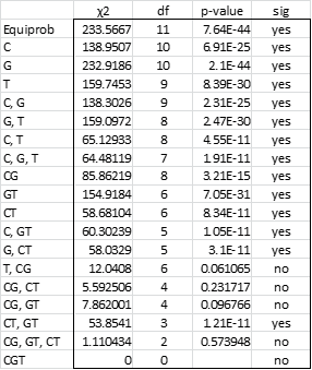
Example 1: Now let us return to the problem we posed in Example 1 of Three-way Contingency Tables, namely to find the most parsimonious model that fits the data. Figure 1 summarizes the key results for all 18 models.

Figure 1 – Summary of all log-linear regression models

From Figure 1, we see that (CGT), (CG, GT, CT), (CG, GT), (CG, CT) and (T, CG) are the only models that fit the data, i.e. provide expected cell frequencies that are not significantly different from the observed cell frequencies. We now describe how to determine which of these models is the most parsimonious.

Observation

If model M₁ has chi-square statistic (maximum likelihood) of χ₁² with df₁ degrees of freedom and model M₂ has chi-square statistic (maximum likelihood) of χ₂² with df₂ degrees of freedom, then

Suppose M₁ and M₂ both provide a significant fit for the observed data and there is no significant difference between χ₁² and χ₂² then if M₂ is a simpler model than M₁ we could just as well use M₂ to model our data as M₁.

Example (continued)

Clearly the saturated model (CGT) is a perfect fit for our data, but, using the above observation, we would like to find a simpler model (one with fewer terms) that is not significantly different from the saturated model.

Of the five models that fit the data, the next most complex model is (CG, GT, CT). The difference between the chi-square statistics for the two models is 1.11 – 0 = 1.1. Since the p-value for 1.11 with 2 – 0 = 2 degrees of freedom is .57 > .05, we conclude there is no significant difference between the two models. This indicates that the interaction between all the variables does not make a significant contribution.

We next compare (CG, GT, CT) with (CG, GT). The difference in the statistics is 7.86 – 1.11 = 6.75, which yields a p-value of .034 on 4 – 2 = 2 degrees of freedom. This is a significant difference, and so we don’t consider (CG, GT) further.

We next compare (CG, GT, CT) with (CG, CT). The difference in statistics is 7.86 – 1.11 = 6.75, which yields a p-value of .106 on 4 – 2 = 2 degrees of freedom. This is not a significant difference, and so we now adopt the simpler model (CG, CT). This indicates that the interaction between G (gender) and T (therapy) does not make a significant contribution.

There is only one other qualifying model to consider, namely (T, CG). The difference in statistics is now 12.04 – 7.86 = 4.18, which yields a p-value of .0398 on 4 – 2 = 2 degrees of freedom. This is a significant difference, and so we reject the (T, CG) model. This indicates that the interaction between C (cure) and T (therapy) does make a significant contribution.

Conclusion

We conclude that (CG, CT) as the simplest (i.e. most parsimonious) model that significantly fits the data.

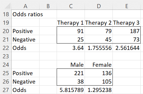
This indicates that there is an interaction between cure and gender as well as between cure and therapy. This can be seen by looking at the odds ratios of the observed data (see Figure 2).

Figure 2 – Odds ratios

That there is an interaction between Cure and Therapy can be seen from the fact that the odds of a cure for therapy 1 is 91/25 = 3.64, while that for therapy 2 is 79/45 = 1.76. The odds ratio is 2.07, i.e. therapy 2 seems to be twice as effective as therapy 1.

That there is an interaction between Cure and Gender can be seen from the fact that the odds of a cure for males is 221/38 = 5.82, while that for females is 136/105 = 1.30. The odds ratio is 4.49, i.e. the therapies seem to be much more effective for men than for women.

Model coefficients

Finally, we calculate the coefficients of the log-linear model for (CG, CT)

using the following coding of the categorical variables:

t_C = 1 if cured and = 0 otherwise
t_G = 1 if male and = 0 otherwise
t_T1 = 1 if therapy 1 and = 0 otherwise
t_T2 = 1 if therapy 2 and = 0 otherwise

It is relatively easy to calculate the coefficients for this model, as described in Figure 3.

Figure 3 – Coefficients for (CG, CT) model

Alternatively, we can use Excel’s regression data analysis tool using L5:L17 as the Y range and D5:J17 as the X range. The coefficients outputted are the same as those given in Figure 3. The rest of the output from the data analysis tool should be ignored.

Thus the log-linear model is

Examples Workbook

Click here to download the Excel workbook with the examples described on this webpage.

Reference

Howell, D. C. (2010) Statistical methods for psychology (7^th ed.). Wadsworth, Cengage Learning.
https://labs.la.utexas.edu/gilden/files/2016/05/Statistics-Text.pdf