We consider simple approaches for using Monte Carlo simulation to estimate the area under a curve y = h(x), bounded by the x-axis and the vertical lines x = a and x = b (see Continuous Probability Distribution). For those familiar with calculus, this is equivalent to estimating the definite integral  dx")
Estimation of Expectation
Suppose that the probability distribution function (pdf) of a distribution is f(x). You can use simulation to estimate the expectation for g(x), including the mean (where g(x) = x).
The expectation of g(x) is defined to be the area under the curve y = g(x)f(x) and above the x-axis, denoted
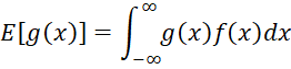
If you draw a random sample x1, …, xn from a distribution with pdf f(x), then, based on the Law of Large Numbers and the Central Limit Theorem, for n large enough
![]()
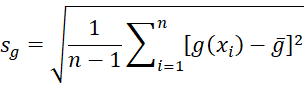
We can also calculate the confidence interval of this estimate as
![]()
where NORM.S.INV(1-α/2,TRUE) ≈ 1.96 and
![]()
and in this way choose a sample size n sufficiently large so that zcrit ⋅ s.e. < ε for a sufficiently small value of ε.
Note too if f(x) is a pdf which is defined only on the interval (a,b) where a can take a finite value or -∞, and b can take a finite value or ∞, then this approach can be used to estimate
Example 1: Find the mean and variance of the beta distribution Bet(2,6).
To estimate the mean, we generate a random distribution x1, …, xn where n = 1,000 from a beta distribution, as described above, and use the function g(x) = x. The results are shown in Figure 1 (only the first 5 elements in the sample are displayed).

Figure 1 – Mean via Monte Carlo
Each of the random values in range B10:B1009 is calculated by the formula =BETA.INV(RAND(),B$3,B$4). The mean of the beta distribution (cell B7) is then estimated as the mean of the g(xi) values in column C. Note that this value, .250641), is quite close to the theoretical mean value, namely α/(α+β) = 2/8 = .25.
We use the fact that the variance is equal to E[x2] – μ2. Figure 1 shows how to calculate the mean μ2. We now use the same approach to find E[x2], this time with g(x) = x2. In fact, we can use the same random values that we generated in Figure 1. The results are shown in Figure 2.

Figure 2 – Variance via Monte Carlo
E[x2] is estimated by the Monte Carlo procedure to be .08434 (cell B8). Combining this result with the mean of .250641 (cell B6) from Figure 1, we obtain a variance of .021553 as shown in cell B9. Note that this is quite similar to the actual variance (cell B7) of

Definite Integral
We can use this method to find the integral of any definite integral  dx")
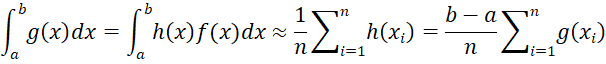
where x1, …, xn is a random sample from the uniform distribution on (a, b)
This approach won’t work when a = -∞ or b = ∞ since in this case, there is no uniform distribution on the interval (a, b).
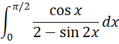
Example 2: Evaluate the definite integral
We use the Monte Carlo approach described above, employing 1,000 simulations. The results are shown in Figure 3.

Figure 3 – Monte Carlo Integration
The estimated value for the definite integral is .785244 (cell B7). Note that the actual value, using analytic techniques is π/4 ≈ .785398 (see Stack Exchange reference below for the details), a difference of .00014 or 0.02%.
Cumulative Distribution
We now extend the Monte Carlo approach to the situation where we know the pdf of a distribution (or at least how to draw random elements from this distribution) and want to estimate the cdf of this distribution at some value b. This is equivalent to estimating

where f(x) is the pdf. This time, we use the function
![]()
We generate a random sample x1, …, xn from the specified distribution and note that

Example 3: Find the cdf value at 1 for the normal distribution with mean 0 and standard deviation 2.
We use the Monte Carlo approach described above, as shown in Figure 4. Since NORM.DIST(2,0,1,TRUE) = .691462 (cell B7), we expect that the estimated value will be near .691462.

Figure 4 – Estimate the cdf using Monte Carlo
We generate a random sample x1, …, xn from the normal distribution with mean 0 and standard deviation 2 using the formula =NORM.INV(RAND(),B$3,B$4) in range B11:B1010 (only the first 5 elements are displayed in Figure 4) and then estimate the cdf at 1 by counting the number of ones in column C and dividing by n = 1,000. This yields a cdf of .675 as shown in cell B8. The value is close to the true value shown in B7. We expect that we will get a more accurate result if we increase the size of the random sample.
Examples Workbook
Click here to download the Excel workbook with the examples described on this webpage.
Reference
Liu, H. and Wasserman, L. (2014) Chapter 12 – Bayesian Inference. Statistical Machine Learning
http://www.stat.cmu.edu/~larry/=sml/Bayes.pdf
Stack Exchange (2016) Compute integral
https://math.stackexchange.com/questions/1820913/compute-int-0-pi-2-frac-cosx2-sin2xdx/1820925#1820925