On this webpage, we augment the results from Conjugate Priors Normal Distribution by using Monte Carlo simulation.
Priors
Example 1: Suppose we believe that the Air Quality Index (AQI) for our city is 40 (towards the end of the good range) with an estimated variance of 100 based on 20 samples based on some historical data. Assuming that our prior has Normal-InverseGamma distribution, use Monte Carlo simulation to develop some intuition about the prior (in order to see whether this prior is representative of our prior beliefs).
The results are shown in Figure 1 based on 10,000 simulations (only the first 5 of the simulations are displayed).
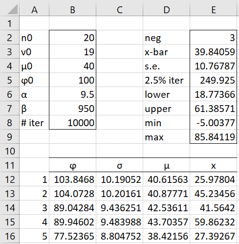
Figure 1 – Simulation of the priors
Representative formulas from Figure 1 are shown in Figure 2.
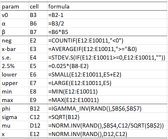
Figure 2 – Representative formulas
We see that the simulated AQI mean (cell E4) is 39.84 (E3), which is not far from the proposed prior mean (cell B4). Note that based on the simulation, the 95% credible interval for the AQI is (18.8, 61.4), which shows the range of credible AQI values (for example on different days) based on our prior beliefs. Note too that the AQI cannot cell be negative, and so we should expect very few if any negative simulated AQI values. From cell E2, we see that only 3 of the 10,000 values are negative, which is a good sign. We excluded these three negative values from the calculation of the 95% credible interval.
Using the Real Statistics Histogram data analysis tool, we see that from Figure 3 that the simulated AQI values do trace out a bell curve as expected.

Figure 3 – Histogram for AQI simulation
Posterior
We can also use Monte Carlo simulation to estimate the values of various posterior parameters. In particular, we will extend the results of Example 1 of Conjugate Priors Normal Distribution, as described in the following example.
Example 2: Suppose our prior beliefs are as described in Example 1 above and using Property 3 of Conjugate Priors Normal Distribution, we obtain a posterior Normal-Gamma distribution with the parameters shown in range B2:B5 of Figure 4. Estimate the (posterior) standard error of the AQI.
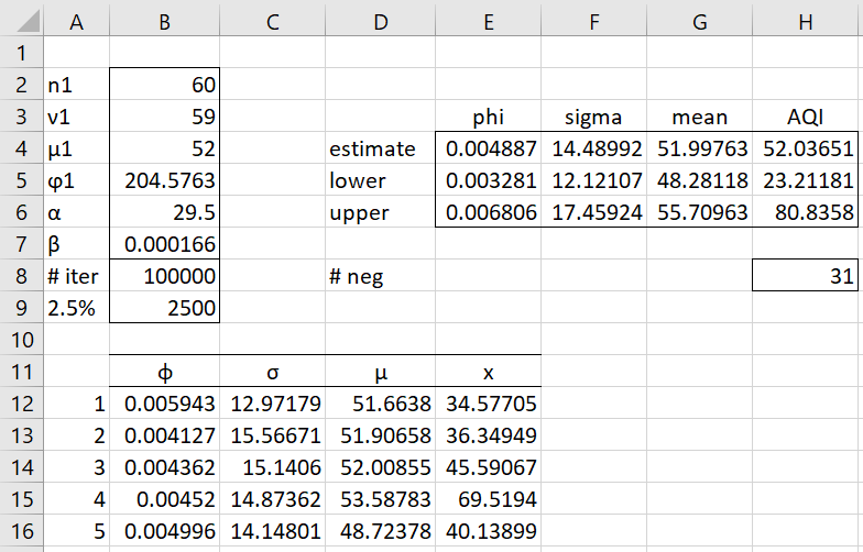
Figure 4 – Posterior Monte Carlo Estimation
We begin by creating 100,000 simulated values for ϕ = 1/φ based on the fact that
![]()
From these simulations, we obtain the corresponding values of the standard errors σ = √φ. Range B12:B100011 contains the simulated values for ϕ and range C12:C100011 contains the simulated values for the standard errors (only the first five values are displayed in Figure 4). Representative formulas used in Figure 4 are shown in Figure 5.
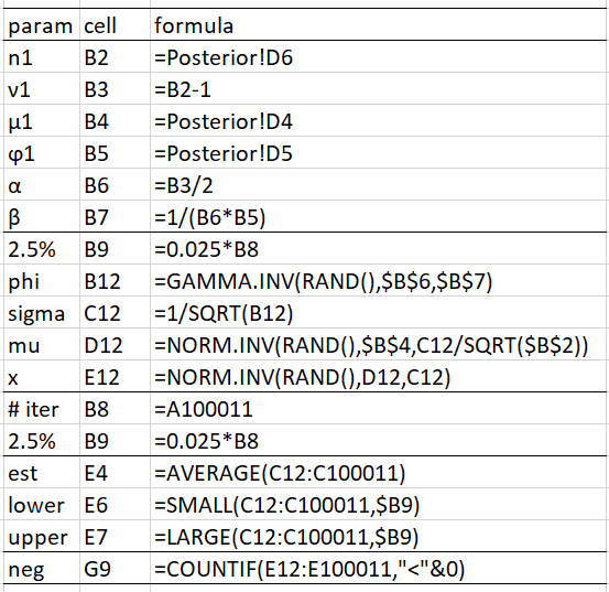
Figure 5 – Key formulas from Figure 4
The values of n1, ν1, μ1, ϕ1, α1, β1 are taken from Figure 4 (Posterior is the name of the spreadsheet shown in Figure 1 of Conjugate Priors Normal Distribution). The average of the 100,000 simulated ϕ and σ values become our estimate of the precision and the standard error, namely .004893 and 14.49, as shown in cells E4 and F4. Note that the estimate for the precision ϕ of .004887 is quite accurate since the theoretic value is the mean of the gamma distribution, namely αβ = 29.5 ∙ .000166 = .004888. The theoretical value for σ = 1/√.004888 is also quite close to the simulated estimate of 14.49.
Credible Interval
In a simulation of 100,000 elements, we can obtain a 95% credible interval by finding the 2.5% × 100,000 = 2,500th (cell B9) smallest and largest values. Thus, (.003281, .006806) is a 95% credible interval for the precision and (12.12, 17.46) is a 95% credible interval for the standard error.
The theoretical 95% credible interval for the precision of (.003286, .006803) can be obtained by using the worksheet formulas =GAMMA.INV(.025, 29.5, .000166, TRUE) and =GAMMA.INV(.975, 29.5, .000166, TRUE). As you can see, the simulated values are quite accurate. Increasing the number of iterations in the simulation will tend to increase the accuracy of the result.
Posterior Mean
Example 3: Estimate the (posterior) mean of the AQI based on the prior and data in Example 2 using simulation.
From range F4:F6 of Figure 5, we see that the Monte Carlo simulation estimate of the AQI mean is 51.998 with a 95% credible interval of (48.28, 55.71). From Property 5 of Conjugate Priors Normal Distribution, the theoretical mean is μ1 = 52 and by Property 4 of that same webpage, (48.31, 55.69) is a 95% credible interval (actually, the HDI) based on the formulas =μ1 ± T.INV.2T(.05, ν1)*SQRT(ϕ1/n1). Again, we see that the simulated estimates are quite close.
We can also obtain a simulated estimate for the AQI of 52.037, as shown in cell H4. This is close to the theoretical value of 52 (equal to the mean). We can obtain a 95% credible interval of (23.21, 80.84) by using the formulas =SMALL(F12:F100011,$B9) and =LARGE(F12:F100011,$B9).
Note that 31 of the simulated AQI values are negative (cell H8). Since the value of the AQI can never be negative, we should not take these 31 negative values into account. Although for this example, 31 out of 100,000 iterations won’t make much of a difference. In any case, we could change the worksheet formulas in cells H4, H5, and H7 to =AVERAGEIF(E12:E100011,”>=”&0), =SMALL(E12:E100011,0.025*(B8-H8)+H8) and =LARGE(E12:E100011,0.025*(B8-H8)).
Example 4: Based on the simulation for Example 3, what is the probability that AQI will exceed 50 (putting the city into the moderate, or higher, category)?
We use the formula =COUNTIF(E12:E100011,”>”&50)/(B8-H8) to obtain the value 55.6%.
Examples Workbook
Click here to download the Excel workbook with the examples described on this webpage.
Reference
Clyde, M., Çetinkaya-Rundel M., Rundel, C., Banks, D., Chai, C., Huang, L. (2019) An introduction to Bayesian thinking
https://statswithr.github.io/book/inference-and-decision-making-with-multiple-parameters.html
AirNow (2021) Air quality index (AQI) basics
https://www.airnow.gov/aqi/aqi-basics/