Gibbs Sampler Algorithm
As described in Gibbs Sampler Two Sample Binomial, suppose we want a sample from the joint distribution f(θ, φ), but we don’t have access to this distribution directly, although we do have access to the distributions for θ|φ and φ|θ. In this case, we can use the following iteration method, called Gibbs Sampler.
- Start with a guess θ0 (which is any permissible value for θ)
- For each i > 0, get sample values θi ∼ f(θ|φi-1) and φi ∼ f(φ|θi)
Then for sufficiently large i, (θi, φi) ∼ f(θ, φ).
Gibbs Sampler for bivariate normal distribution
Example 1: Create a sample of size 2,000 from a bivariate normal distribution with μ1 = 2, μ2 = 1, σ1 = .5, σ2 = 1.5 and ρ = .6 using Gibbs Sampler.
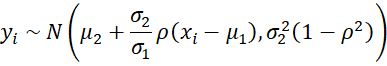
We create a sample of 2,100 points (xi, yi) where we throw away the first 100 values. We start with an initial values for x0 and y0 of zero, and then at each iteration, we look for random values such that

The result is shown in Figure 1 where only the first eight of 2,100 sample pairs (xi, yi) are displayed in columns H and I, and where range B2:B6 shows the target parameters of the desired bivariate normal distribution.
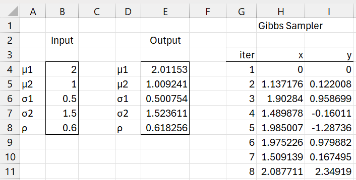
Figure 1 – Gibbs Sampler for bivariate normal distribution
Representative Formulas
Representative formulas from Figure 1 are shown in Figure 2. Range E2:E6 shows the calculated parameter values based on the sample generated in range B109:C2108. We see that these values are fairly close to the values in range B2:B6, as expected.
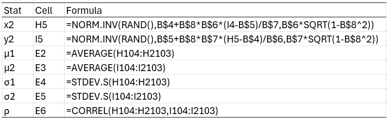
Figure 2 – Representative formulas from Figure 1
Data Analysis Tool
We can obtain a similar result by using Real Statistics’ Gibbs Sampler data analysis tool.
This is done by pressing Ctrl-m and selecting the Gibbs Sampler option from the Bayes tab. You next fill in the dialog that is displayed as shown in Figure 3.
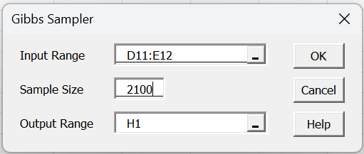
Figure 3 – Gibbs Sampler dialog box
Here the Input Range refers to a 2 × 2 range with the following entries:
Cell 1,1: initial x guess
Cell 1,2: initial y guess; numeric value
Cell 2,1: pdf formula at x for y in cell 1,2
Cell 2,2: pdf formula at y for x in cell 2,1
For Example 1, this input range is shown in range D11:E12 of Figure 4.
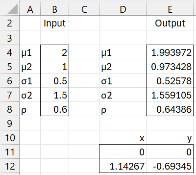
Figure 4 – Input range for Example 1
Here cells D12 and E12 contain the formulas
=NORM.INV(RAND(),B$4+B$8*B$6*(E11-B$5)/B$7,B$6*SQRT(1-B$8^2))
=NORM.INV(RAND(),B$5+B$8*B$7*(D12-B$4)/B$6,B$7*SQRT(1-B$8^2))
These are similar to the formulas in cells H5 and I5 of Figure 2. It is important that any cell references to the initial guesses for y and the first calculated x cell (cells E11 and D12) use relative addressing (i.e. contain no $ signs) and any references to other cells use absolute addressing (i.e. contain a $ sign).
After pressing the OK button on the dialog box the output will be similar to that shown in Figure 1.
Caution: The Help for the Gibbs Sampler data analysis tool states that the input range consists of a column range with three rows. This is incorrect. It consists of a 2 × 2 range as described above.
Examples Workbook
Click here to download the Excel workbook with the examples described on this webpage.
References
Peng, R. D. (2021) Advanced statistical computing
https://bookdown.org/rdpeng/advstatcomp/
https://bookdown.org/rdpeng/advstatcomp/gibbs-sampler.html#example-bivariate-normal-distribution
https://bookdown.org/rdpeng/advstatcomp/gibbs-sampler.html#example-normal-likelihood