Since the normal distribution is defined by two parameters, the mean and variance, we describe three types of conjugate priors for normally distributed data: (1) mean unknown and variance known, (2) variance unknown and mean known, and (3) mean and variance are unknown.
Unknown mean and known variance
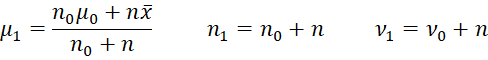
Property 1: If the independent sample data X = x1, …, xn follow a normal distribution with a known variance φ and unknown mean µ where X|µ ∼ N(µ, φ) and the prior distribution is µ ∼ N(µ0, φ0), then the posterior µ|X ∼ N(µ1, φ1) where
![]() Proof: Click here
Proof: Click here
Property 2: If the independent sample data X = x1, …, xn follows a normal distribution with known variance φ and unknown mean µ where X|µ ∼ N(µ, φ) and the prior distribution is µ ∼ N(µ0, φ0), then the posterior µ|X ∼ N(µ1, φ1) where
![]()
Proof: This property follows from Property 1 since
![]()
Unknown variance and known mean
Property 2: If the independent sample data X = x1, …, xn follow a normal distribution with an unknown variance φ and a known mean µ where X|φ ∼ N(µ, φ) and the prior distribution is φ ∼ Scaled-Inv-χ2(ν0, s02) with scale parameter s02 and degrees of freedom ν1 > 0, then the posterior φ|X ∼ Scaled-Inv-χ2(ν1, s12) where
![]()
![]()
Proof: Click here
See Bayesian Distributions for a description of the scaled inverse chi-square distribution. Also, note that the following are equivalent:
- x ∼ Scaled-Inv-χ2(ν, s2)
- x ∼ Inv-Gamma(ν/2, νs2/2)
- 1/x ∼ Gamma(ν/2, 2/(νs2))
Unknown mean and variance
Generally, both the mean and variance are unknown, and so the approach is more complicated than that described by Properties 1 and 2. In particular, we need to look at the case where the data comes from a normal distribution with unknown mean µ and unknown variance φ. As a result, we need to consider the joint probability f(µ, φ) and the likelihood function l(µ, φ|X) and use the following form of Bayes Theorem:
![]()
If we let ϕ = 1/φ, then we can use ϕ ∼ Gamma(ν0/2, ν0φ0/2) as the prior distribution for ϕ. Here, φ0 may be viewed as the prior estimate for the variance φ = 1/ϕ and ν0 may be viewed as the prior estimate of the degrees of freedom (for the chi-square estimate of the variance).
We can use μ|φ ∼ N(μ0, φ*) as the prior estimate for the mean (conditional on the variance φ). Since μ is conditional on φ, we can assume in this context that φ is known and so the variance φ* can be expressed as φ/n0 for some unknown parameter n0. Thus, the prior takes the form μ|φ ∼ N(μ0, φ/n0), which is equivalent to μ|ϕ ∼ N(μ0, 1/(n0ϕ)),
Note that in what follows, n0 can be interpreted as the sample size of some assumed prior distribution.
Normal-Gamma Distribution
Definition 1: The joint distribution of μ, ϕ has a normal-gamma distribution, denoted
![]()
provided

In what follows, φ will represent a variance parameter and ϕ = 1/φ, also called the precision.
Definition 2: The joint distribution of μ, φ has a normal-inverse chi-square distribution, denoted
![]()
provided
![]()
Here, φ has a scaled inverse chi-square distribution (see Bayesian Distributions).
Note that μ, φ ∼ Norm-χ2(μ0, n0, φ0, ν0) is equivalent to μ, 1/φ ∼ NormGamma(μ0, n0, φ0, ν0).
Key Property
Property 3: If the independent sample data X = x1, …, xn follow a normal distribution with an unknown mean µ and variance φ where X|µ, φ ∼ N(µ, φ) and
![]()
with ϕ = 1/φ, then the posterior is
![]()
where

Proof: Click here
Example
Example 1: Suppose our prior belief, based on historical data, is that the Air Quality Index (AQI) for our city is 40 (towards the end of the good range) with an estimated variance of 100 based on 20 samples. We now take 40 samples of the air quality and observe a mean of 58 (in the lower end of the moderate range for AQI) and a variance of 150. Find the posterior distribution using Property 3.
The posterior parameters are
![]()
![]()
![]()
![]()
![]()
The calculations are shown in the upper part of Figure 1.
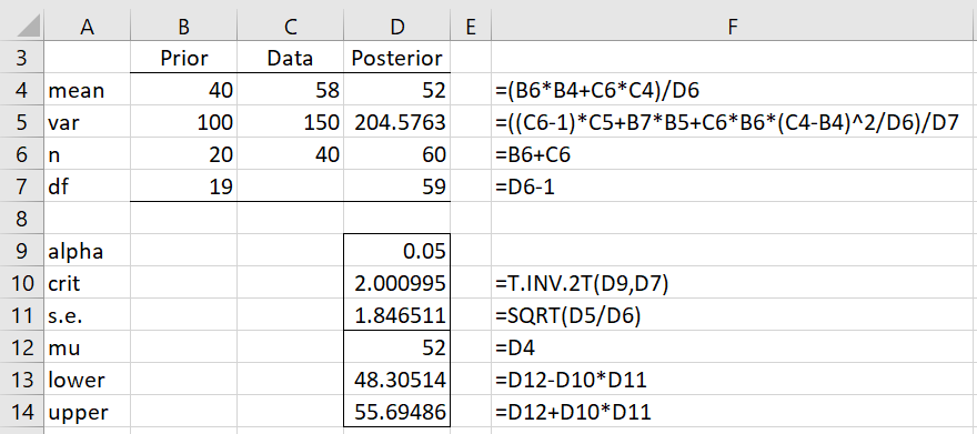
Figure 1 – Posterior distribution
Worksheet Function
Real Statistics Function: The Real Statistics Resource Pack supports the following array function.
NORM_GAMMA(x̄, s2, n, μ0, φ0, n0, lab): returns a column array with the posterior values μ1, φ1, n1. If lab = TRUE (default FALSE), then an extra column of labels is appended to the output.
The output for the formula =NORM_GAMMA(C4,C5,C6,B4,B5,B6) is shown in range D4:D6 of Figure 1.
More Properties
Property 4: If the independent sample data X = x1, …, xn follow a normal distribution with an unknown mean µ and variance φ where X|µ, φ ∼ N(µ, φ) and
![]()
with ϕ = 1/φ, then the marginal distribution of μ is
Proof: Click here
Property 5: Given the premises of Property 4, it follows that for ν0 > 1, the mean of μ is μ0
Proof: Click here
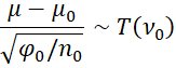
HDI Interval
Since the t-distribution is unimodal and symmetric, the 1-α HDI interval for μ can be expressed as
![]()
![]()
where tcrit = T.INV.2T(α, ν0). Note that in this formulation, unlike in the frequentist approach, the probability that the population mean μ is in the HDI is 1-α.
Observation: Properties 4 and 5, as well as the previous observation, holds for both the prior (as stated) as well as for the posterior.
Example 2: What is the expected posterior value of μ in Example 1 and what is the 95% HDI?
By Property 5, the expected posterior value for the mean is μ1 = 52 and the 95% HDI is
![]()
which, as shown in the lower part of Figure 1, yields a 95% HDI of (48.3, 58.7). Thus, it is 95% likely that the AQI will be in this range. Most of this interval is in the moderate part of the AQI range.
Examples Workbook
Click here to download the Excel workbook with the examples described on this webpage.
References
Clyde, M., Çetinkaya-Rundel M., Rundel, C., Banks, D., Chai, C., Huang, L. (2019) An introduction to Bayesian thinking
https://statswithr.github.io/book/inference-and-decision-making-with-multiple-parameters.html
Walsh, B. (2002) Introduction to Bayesian Analysis
http://staff.ustc.edu.cn/~jbs/Bayesian%20(1).pdf
AirNow (2021) Air quality index (AQI) basics
https://www.airnow.gov/aqi/aqi-basics/