Objective
We show how to perform hypothesis testing for normally distributed data using the Bayesian approach described at Bayesian Hypothesis Testing.
On this webpage, we focus on the following one-sided tests using non-informative priors. Since we use non-informative priors, the Bayes factors are not defined, and so we specify the posterior odds instead.
- One sample test with
- known variance
- unknown variance
- Two sample test
- equal fixed variance
- equal unknown variance
- unequal unknown variances
Click here for a description the two-sided versions of these hypothesis tests.
Click here for a description of Excel worksheet functions and data analysis tools supplied by the Real Statistics Resource Pack that implement the tests described on this webpage.
One-sample test with known variance
Suppose we have a sample X = x1, …, xn that comes from a normally distributed population with known fixed variance; i.e. xi ~ N(μ, σ2) for all i. We test the following null and alternative hypotheses.
H0: μ < 0
H1: μ ≥ 0
We assume the Jeffreys’ prior f(μ) ∝ 1 (see Non-informative Priors). Thus, the posterior is proportional to the likelihood function, and so
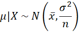
The posterior probability of the null-hypothesis is therefore
![]()
where Φ is the cdf for the standard normal distribution and
![]()
If your decision criterion for rejecting H0 in favor of H1 is that P(H0|X) < α, then you can use the frequentist one-sided z-test, namely reject the null hypothesis if –z < zα or equivalently +z > z1-α.
Example 1: The data in Figure 1 is normally distributed with known variance 125. Test the null hypothesis that μ < 25 vs. the alternative hypothesis μ ≥ 25.
We first subtract 25 from the data and test whether μ ≥ 0 on the revised data. We see that P(H1|X) = .0706575 (cell E11) and Odds01 = 13.149 (cell E12), which is strong evidence in support of the null hypothesis.
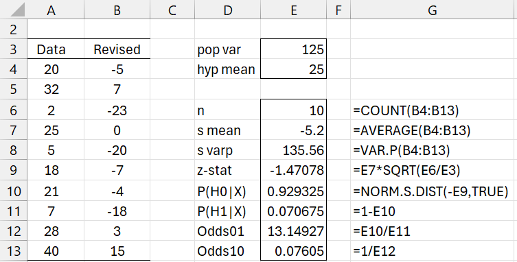
Figure 1 – Bayesian one-sample z-test
Note that we obtain the same results using the original data and subtracting the hypothetical mean from the sample mean in the above calculations.
One-sample test with unknown variance
We repeat the above one-sided test where the variance is unknown. This time we use the Jeffreys’ prior
f(μ, σ) = σ-3
(see Non-informative Priors). The resulting posterior for μ is
![]()
where tn is the non-standardized t-distribution. tν(µ, σ2) is referred to as T(ν, µ, σ) on that webpage.
This is the same as the usual frequentist t-test except that s2 is defined with division by n instead of n-1, and the degrees of freedom is n instead of n-1.
Click here for a proof of the above assertion.
Example 2: Repeat Example 1 where the variance is estimated from the sample.
We see from Figure 2 that P(H1|X) = .094103 (cell E10) and Odds01 = 9.626597, which is reasonably strong evidence in support of the null hypothesis.
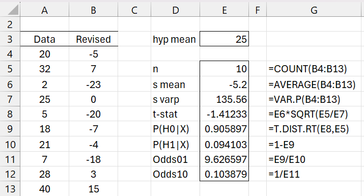
Figure 2 – Bayesian one-sample t-test
Note that P(H0|X) can also be calculated via the worksheet formula =T3_DIST(0,E6,E7,SQRT(E8/E6),TRUE) and P(H1|X) can be calculated via the formula =T3_DIST(E7,E6,0,SQRT(E8/E6),TRUE) .
Two-sample test with equal known variance
Suppose we have a samples X = x1, …, xm and Y = y1, …, yn that comes from a normally distributed population with known fixed variance; i.e. xi ~ N(μx, σ2) and yi ~ N(μy, σ2) for all i. We test the following null and alternative hypotheses where δ = μy – μx.
H0: μx > μy (or δ < 0)
H1: μx ≤ μy (or δ ≥ 0)
We use the Jeffreys’ prior f(μx, μy) = 1. It can be shown that the posterior distribution is
![]()
Once again, this takes the form of the frequentist test with a cleaner interpretation.
Two-sample test with equal unknown variances
This time we use the Jeffreys’ prior f(μx, δ, σ2) ∝ (σ2)-2. It turns out that the posterior (calculated by integrating over μx and σ2) is
![]()
where the pooled variance is
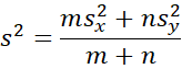
with
![]()
Example 3: Test the null hypothesis μNew > μOld vs. the alternative hypothesis μNew ≤ μOld based on the data in Figure 3.
The analysis is shown in Figure 3. This time, the evidence favors the alternative hypothesis, but just barely since Odds10 = 1.105. Column I shows the formulas in column G.
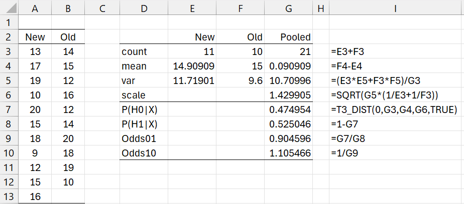
Figure 3 – Bayesian two-sample t-test
Two-sample test with unequal unknown variances
Since neither group shares any parameters, we can use the one sample approach to obtain
![]()
Example 4: Repeat Example 2 of Two Sample t Test: Unequal Variances using a Bayesian approach. The data for this example is shown in range A3:B13 of Figure 4.
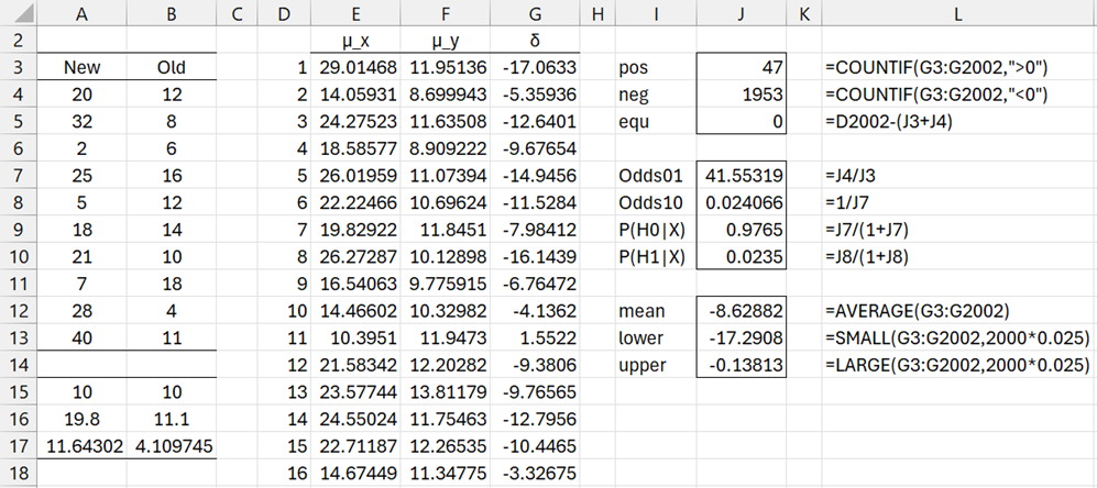
Figure 4 – Two sample hypothesis test using simulation
We use Monte Carlo simulation with 2,000 iterations as shown in Figure 4. First we calculate the size, mean, and standard deviation for the two samples, as shown in range A15:B17. This is done by placing the formulas COUNT(A3:A13), AVERAGE(A3:A13, and STDEV.P(A3:A13) in cells A15, A16, and A17. We then highlight range A15:B17, and press Ctrl-R.
Next, we insert the formula =A$16+A$17/SQRT(A$15)*T.INV(RAND(),A$15) in cell E3, highlight range E3:F2002, and press Ctrl-R and Ctrl-D. This yields samples X and Y from two t-distributions with the parameters corresponding to the samples in columns A and B. Next, we obtain the values for δ by placing the formula =F3-E3 in cell G3, highlighting G3:G2002, and pressing Ctrl-D.
Finally, we obtain the counts for δ > 0 and δ ≤ 0, namely 47 and 1953, as shown in cells J3 & J4. From this simulation, we see that P(H0|X,Y) = 1953/2000 = .9765 and P(H1|X,Y) = 47/2000 = .0235.
The simulation also produces an estimated 95% credible interval of (-17.20, -.138) for the mean, as shown in range J13:J14).
We see that data favors the null hypothesis with posterior Odds01 = .9765/.0235 = 41.55319 (cell J7), which indicates that the difference between the two samples is quite strong per Figure 1 of Bayesian Hypothesis Testing.
Note too that we could also get the simulated data in Figure 4 by inserting the formula =T3_INV(RAND(),A$15, A$16, A$17/SQRT(A$15)) in cell E3. Finally, note that we could get a more accurate result by increasing the number of simulations.
Examples Workbook
Click here to download the Excel workbook with the examples described on this webpage.
References
Reich, B. J., Ghosh, S. K. (2019) Bayesian statistics methods. CRC Press
Lee, P. M. (2012) Bayesian statistics an introduction. 4th Ed. Wiley
https://www.wiley.com/en-us/Bayesian+Statistics%3A+An+Introduction%2C+4th+Edition-p-9781118332573
Jordan, M. (2010) Bayesian modeling and inference. Lecture 1. Course notes
https://people.eecs.berkeley.edu/~jordan/courses/260-spring10/lectures/lecture1.pdf
Gelman, A., Carlin, J. B., Stern, H. S., Dunson, D. B., Vehtari, A., Rubin, D. B. (2014) Bayesian data analysis, 3rd Ed. CRC Press
https://statisticalsupportandresearch.files.wordpress.com/2017/11/bayesian_data_analysis.pdf
Clyde, M. et al. (2022) An introduction to Bayesian thinking
https://statswithr.github.io/book/_main.pdf