Random Walk Metropolis Algorithm

Basic Concepts

Suppose we want to estimate the posterior distribution P(θ|X) or at least generate values for θ from this distribution.

• Start with a guess θ₀ for θ in the acceptable range for θ.
• For each i ≥ 0

(a) Get a random value θ′_i+1 ∼ J(θ_i, φ)

(b) Set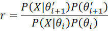

although if θ′_i+1 is outside the acceptable range for θ then set r = 0

(c) Get a random value u between 0 and 1

(d) If r > u, then set θ_i+1 = θ′_i+1; otherwise set θ_i+1 = θ_i

J(θ, φ) is called the proposal distribution (aka the jump distribution), φ is called the step parameter and θ′_i+1 is called the proposed value of θ at iteration i+1. Note that if r > 1, then it will always be the case that θ_i+1 = θ′_i+1.

The Metropolis algorithm is based on a Markov chain with an infinite number of states (potentially all the values of θ). Note that r is simply the ratio of P(θ′_i+1|X) with P(θ_i|X)  since by Bayes Theorem

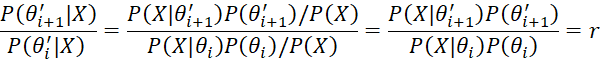
Since values of P(X) cancel out, we don’t need to calculate P(X), which is usually the most difficult part of applying Bayes Theorem.

Observation: We can use the Metropolis algorithm to estimate the posterior distribution for the problem of flipping a coin n times based on the binomial distribution with a beta prior Bet(α, β).

We choose as our proposal distribution a normal distribution N(θ, σ²). Thus, we can consider θ′_i+1 = θ_i + Δθ where Δθ ∼ N(0,σ²). Since Δθ is normally distributed, about 95% of the time θ′_i+1 will be within two standard deviations of θ_i. σ² can be selected to determine how big a jump we want to make at each step in the iteration.

For a large enough iteration, the sequence θ₁, θ₂, …, θ_k will be a sample from the posterior distribution, however, it isn’t a random sample (since there is a correlation between the elements in the sample), but it will have some nice properties (e.g. the mean of this sequence will converge to the mean of the posterior distribution for large k). To get a random sample of size n, you need to follow use the Metropolis algorithm n times selecting the last (i.e. k^th) value from each sample.

Example of the Algorithm

Example 1: Use the Metropolis algorithm to estimate the mean of the posterior distribution for Example 3 of Beta Conjugate Prior. Thus, we assume a prior beta distribution Bet(4,4) and we have observed 3 heads in 16 tosses of a coin.

We use Δθ ∼ N(0,σ²) with σ = .1. Figure 1 displays the first 10 of a sample of 500 elements generated using the Random Walk Metropolis algorithm. E.g. cell B8 contains the formula =NORM.INV(RAND(),E7,$F$2), cell D8 contains =RAND(), E8 contains =IF(C8>D8,B8,E7), and C8 contains

=IF(AND(B8<1,B8>0),BINOM.DIST($D$3,$D$2,B8,FALSE)* BETA.DIST(B8,$B$2,$B$3,FALSE)/(BINOM.DIST($D$3,$D$2,E7, FALSE)*BETA.DIST(E7,$B$2,$B$3,FALSE)),0)

We see from column H that 169 of the 500 proposed values, p′ for p|X, were not accepted. Of these, 8 of the p′ were negative. The mean value for p|X is .27419, which is pretty close to the theoretical mean value of 7/(7+17) = .29167 for the Bet(7,17) posterior distribution determined using Property 1 of Analytic Approach for Binomial Data. We expect that the larger the sample, the more accurate the results would be.

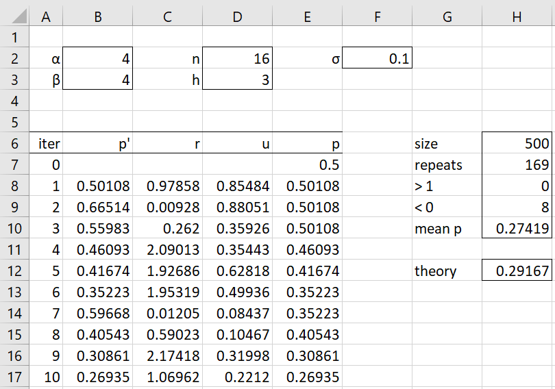
Figure 1 – Metropolis algorithm

In Figure 2, we compare the histogram of the data from the Metropolis algorithm (from Figure 1) with the results expected from a  distribution.

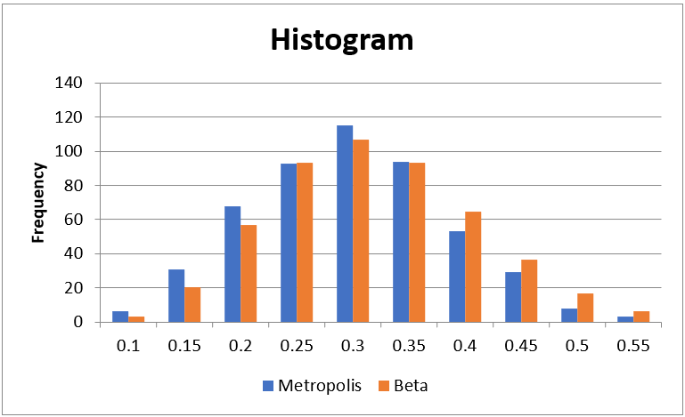
Figure 2 – Comparison of Metropolis vs Beta histograms

Once again, with a larger sample, we would expect an even better match. In fact, more typically we would use a sample of size 10,000 or 50,000 and not count the first 500 elements towards the calculation of the mean, mode, HDI, or whatever information we are interested in. These first elements are eliminated because they are more dependent on the initial guess.

HDI

Example 2: Use the results from Example 1 to estimate a 95% HDI.

The results are shown in Figure 3. Column A contains a copy of the Metropolis sample from range E8:E507 of Figure 2. Column D contains the values in column A in sorted order, e.g. by using the array formula =QSORT(A4:A503). Since .05 · 500 = 25, then, only the first 25+1 = 26 elements in column D can act as potential a values of a 95% credible interval [a, b]. For each of these, the corresponding b value is located 474 rows later. E.g. the b value corresponding to the first a is shown in cell E4, as calculated by the value =INDEX($D$4:$D$503,C4+474). The length of each of these intervals, b–a, is shown in column F. E.g. the length of the first credible interval is shown in cell F4, as calculated by the formula =F4-E4.

Now, the smallest credible interval has a length of .317681, as calculated by the formula =MIN(F4:F29). Note that this value can also be calculated via the following array formula.

=MIN(IFERROR(INDEX($D$4:$D$503,C4:C503+474)-D4:D503,1))

We see that F7 is the only cell in column F that contains the value .317681, and so using the corresponding a and b values, the estimated 95% HDI is [.099063, .416744]. This compares with the more accurate 95% HDI of [.122023, .470874] as calculated in Example 2 of HDI from Posterior Beta. Once again, using a larger Metropolis sample will generally yield more accurate results. The value of the step parameter (σ = .1) for this example) will also impact how quickly or slowly the algorithm converges to a more accurate sample.

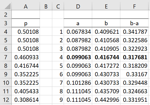
Figure 3 – 95% HDI

Worksheet Function

Real Statistics Function: The Real Statistics Resource Pack supports the following array function.

SAMPLE_HDI(R1, lab, p): returns a column array with the endpoints of the 1–p HDI based on the data in R1; default for p is .05; if lab = TRUE (default FALSE) then a column of labels is appended to the output.

The 95% HDI for Example 2 can also be found using the array formula =SAMPLE_HDI(E8:E507,TRUE), as shown in Figure 4.

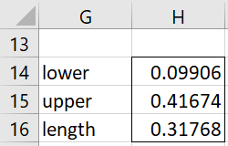
Figure 4 – 95% HDI

References

Gelman, A., Carlin, J. B., Stern, H. S., Dunson, D. B., Vehtari, A., Rubin, D. B. (2014) Bayesian data analysis, 3rd Ed. CRC Press
https://statisticalsupportandresearch.files.wordpress.com/2017/11/bayesian_data_analysis.pdf
Marin, J-M and Robert, C. R. (2014) Bayesian essentials with R. 2nd Ed. Springer
https://www.springer.com/gp/book/9781461486862
Jordan, M. (2010) Bayesian modeling and inference. Course notes
https://people.eecs.berkeley.edu/~jordan/courses/260-spring10/lectures/index.html
Lee, P. M. (2012) Bayesian statistics an introduction. 4th Ed. Wiley
https://www.wiley.com/en-us/Bayesian+Statistics%3A+An+Introduction%2C+4th+Edition-p-9781118332573
Reich, B. J., Ghosh, S. K. (2019) Bayesian statistics methods. CRC Press
Thank you very much Dr.
In the case of wanting to estimate a linear regression model, what would the estimation procedure be like?
Hello Antony,
The following may be useful
https://khayatrayen.github.io/MCMC.html
https://m-clark.github.io/models-by-example/metropolis-hastings.html
https://medium.com/@tinonucera/bayesian-linear-regression-from-scratch-a-metropolis-hastings-implementation-63526857f191