Basic Concepts
Credible intervals are the Bayesian version of confidence intervals. The interpretation of a 1–α confidence interval for a parameter θ is that for 1–α of the samples, the true value of θ will lie in a similarly constructed confidence interval derived from that sample. A 1–α credible interval for a parameter θ means that 1–α is the probability that the true value of θ lies in that interval.
For Example 2 of Grid Estimation, a 95% credible (posterior) interval is one in which 95% of the area under the curve shown in Figure 2 of Grid Estimation is found between the endpoints of the interval. E.g. the interval [.08, .44] is an approximately 95% credible interval. In fact, it is a 94.85% credible interval since SUM(F20,F47) = .9485 (with reference to Figure 2 of Grid Estimation). Another approximately 95% credible interval is [.12, 1] since SUM(F15:F103) = .9522.
In general, we prefer a smaller credible interval to a larger interval. This would favor the [.08, .44] interval over the [.12, 1] interval. In fact, [.09, .45] has the same size as the [.08, .44] interval, but it is a 94.994% credible interval, which is closer to the 95% target. The smallest such interval is called the high density interval (HDI).
When calculating the HDI from a grid, we have two goals: minimizing the length of the interval and obtaining a credible interval as close to the goal (95% in the above example) as possible. The Real Statistics GRID_HDI function, described below, attempts to meet these two goals.
Real Statistics Support
Real Statistics Function: The following array function identifies the 1–p HDI for the x data in R1 and corresponding f(x) pdf data in R2.
GRID_HDI(R1, R2, lab, p, lprec, uprec): returns a column array with the following entries: endpoints of the HDI, length of the HDI and the actual value for 1–p based on the HDI.
If lab = TRUE (default FALSE) a column of labels is appended to the output.
Since a grid is finite, it is likely that there is no 1–p credible interval; instead, we seek a credible interval that is near 1–p. E.g. for a 95% credible interval, it may be acceptable to consider any interval between 94.5% and 95.5%. This is accomplished by setting p = .05 and the lower and upper precision values equal to .1, i.e. lprec = uprec = .1. This is appropriate since (.1)(.05) = .005 and so we accept 1 – pp credible intervals where pp is between .05-.005 = .045 and .05+.005 = .055, i.e. where 1–pp is between 94.5% and 95.5%.
Algorithm
The search algorithm used to identify the HDI tries to find the shortest 1–pp credible interval. If there is more than one such interval, then it selects the one such pp is as close as possible to p.
Note that the values for lprec and uprec don’t have to be equal. In fact, they can be any relatively small non-negative value.
The default value for p is .05 and the default values for lprec and uprec are .1.
We can use this function to find the HDI for the posterior pdf in Figure 2 of Creating a Grid using Real Statistics (where ranges F4:F104 and J4:J104 are as shown in that figure). This is done by inserting the array formula =GRID_HDI(F4:F104,J4:J104,TRUE) in range L3:M6 of Figure 1 below. We see that [.09, .45] is a 94.99% HDI. Note that [.08, .44] is also a potential 95% HDI. Since SUM(J12:J48) = .9485, this is actually a 94.85% HDI, which is farther from 95% than 94.99%, and so we opt for the HDI shown in Figure 1.
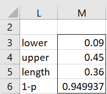
Figure 1 – 95% HDI
Examples Workbook
Click here to download the Excel workbook with the examples described on this webpage.
Reference
Kruschke, J. K. (2015) Doing Bayesian data analysis. 2nd Ed. Elsevier
https://sites.google.com/site/doingbayesiandataanalysis/