Basic concepts
Example 1: Suppose that we want to test whether a coin is fair based on 16 tosses resulting in 3 heads.
In the frequentist approach, we can use a one-tail test (H0: p ≥ .5, H1: p < .5), assuming that we don’t expect the coin to be biased towards tails, based on the binomial distribution with a sample size of n = 16.
Since p-value = BINOM.DIST(3,16,.5,TRUE) = .0106 < .05 = α, we reject the null hypothesis and find that it is likely that the coin is indeed biased. If we perform a two-tailed test (H0: p = .5, H1: p ≠ .5), and so we don’t have any information about the direction of any bias if it exists, then p-value = .0212 < .05 = α, and so once again we see that it is likely that the coin is biased.
Bayesian approach
In the Bayesian approach, we must first determine our prior belief about the probabilities of each of the possible outcomes. Let p = the probability that a random toss will come up heads. A priori, p can take any value between 0 and 1, but to simplify matters we will assume that p can only take the values 0, .1, .2, .3, .4, .5, .6, .7, .8, .9 or 1.
Even so, there are many ways to assign probability values P(p) to these 11 possible outcomes. Assuming we tend to believe that the coin is fair and it is less likely that the extremes will occur, we assign probabilities as shown in column C of Figure 1. This is based on a triangular distribution with a mode at p = .5 (graph in blue).
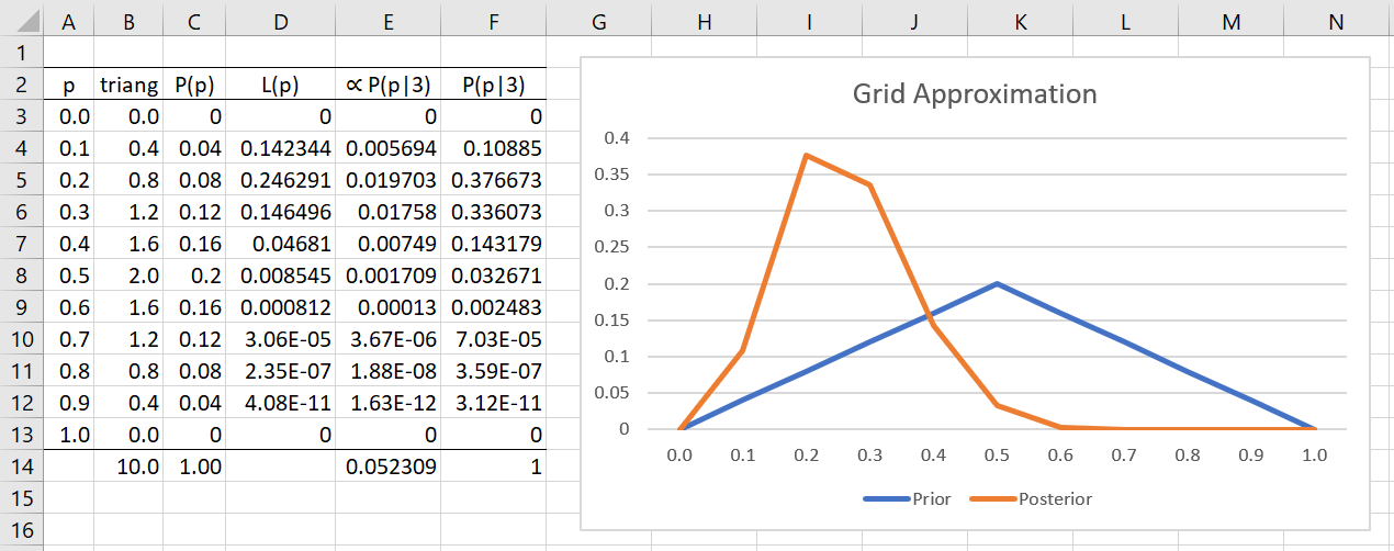
Figure 1 – Estimation of the posterior distribution
Next, we need to calculate the likelihood that 3 out of 16 values are heads conditional on each of the 11 possible p values. This is shown in column D of Figure 1. For example, when p = .1, the likelihood value is calculated by =BINOM.DIST(3,16,A4,FALSE), as shown in cell D4. To obtain the unnormalized posterior probability we multiply the values in column C by the corresponding value in column D to obtain the values shown in column E. These values are proportional to the (normalized) posterior probabilities.
To obtain the posterior probabilities, we add up the values in column E (cell E14) and divide each of the values in column E by this sum. The resulting posterior probabilities are shown in column F.
Results
We see that the most likely posterior probability is p = .2 since the largest value in column F is P(p|3) = 37.7%, which occurs then p = .2.
Note that while we previously believed it most likely that p = .5 (with a probability of 20%), based on the data, this probability has now dropped to 3.3%.
Using the formula =SUM(F3:F7), we also see that the probability that the coin will come up tails more frequently than heads is 96.7%.
Finer grid
Example 2: Repeat Example 1 using a finer grid, namely with values of p = 0, .01, .02, …, .98, .99, 1.
Once again, we use a triangular distribution for our priors (blue chart). The resulting posterior distribution (red) is shown in Figure 2 (only the first 16 of 101 rows are visible, with the column sums in row 104). This time, we see that the most likely posterior probability is p = .24 since the largest value in column F is P(p|3) = 4.02%, which occurs when p = .24. The probability the coin will come up tails more frequently than heads is 98.5%, via the formula =SUM(F3:F52), and the probability that heads will come up more frequently than tails is only 1.2% (the remaining .3% is the probability that heads and tails come up the same number of times).
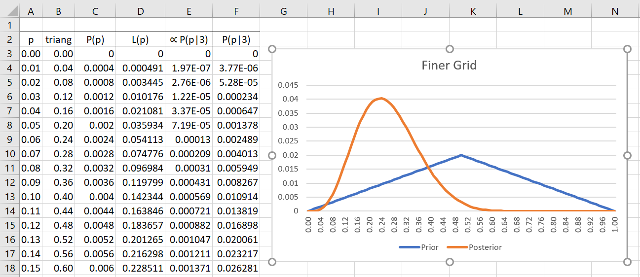
Figure 2 – Estimation using a finer grid
More data
Example 3: Suppose we repeat the experiment from Example 2, but this time with a sample 3 times as large, and suppose that the same proportion of heads results, namely 9 heads (out of 48 tosses). Using the same priors as in Example 2, we get the posterior probabilities shown in red in Figure 3. We also display the posterior probabilities from Example 2 in gray. The only change from Figure 2 is that we place the formula =BINOM.DIST(9, 48, A3, FALSE) in cell D3, highlight the range D3:D103 and press Ctrl-D.
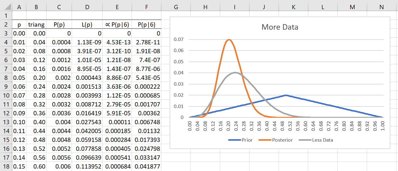
Figure 3 – Estimation using more data
We see that the posterior curve from Example 3 is narrower, with a higher mode, and skewed more to the right than the posterior curve from Example 2. This demonstrates that the more data, the more accurate the estimate (a narrower curve indicates less variance). It also demonstrates that the more data we have, the more the data influences the posterior probabilities and the less the prior probabilities influence the posterior probabilities.
The following web pages have more information about Bayesian grids:
- Creating Bayesian Grids using Real Statistics
- Credible intervals and how to create an HDI using Real Statistics
- Bayesian analysis using grids
Examples Workbook
Click here to download the Excel workbook with the examples described on this webpage.
Reference
Kruschke, J. K. (2015) Doing Bayesian data analysis. 2nd Ed. Elsevier
https://sites.google.com/site/doingbayesiandataanalysis/