Basic Concepts
We show how to determine the posterior distribution for two samples that are binomially distributed assuming a beta prior. E.g. suppose we toss two coins multiple times and we investigate the percentage of heads that we observe from each coin. We will assume that the coins are independent in the sense that these percentages are independent of each other.
Let x = the number of heads that come up in m tosses from coin 1 and let y = the number of heads that come up in n tosses from coin 2. Let f(x, y) = the probability that we observe x heads in m tosses of coin 1 and y heads in n tosses of coin 2. Since this is a joint probability function
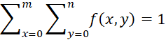
The independence assumption means that
![]()
where f(x) and f(y) are the corresponding marginal probability distributions:
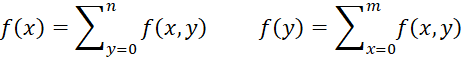
Since we are assuming that x and y follow a binomial distribution, we also need to know what the probability that heads will come up for each coin. As usual, in the Bayesian approach, these are random variables that we will denote as p for coin 1 and q for coin 2. Thus x ∼ Binom(m, p) and y ∼ Binom(n, q).
We will suppose that the prior distribution for p and q is continuous with pdf f(p, q). As usual, we are abusing the notation since f(x, y) and f(p, q) are not the same functions. Since f(p, q) is a pdf, it follows that
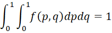
Since we assume that the coins are independent, it follows that
![]()
where f(p) and f(q) are the corresponding marginal pdfs, and so
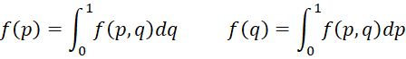
Here, the integrals play the role that the sums played for the discrete f(x, y). If you don’t know calculus, don’t be alarmed because we will avoid using integrals in what follows.
Property
Property 1: Suppose x is the number of successes in m trials, following a binomial distribution with unknown parameter p, and the prior distribution is p ∼ Bet(α, β). Suppose too that y is the number of successes in n trials, following a binomial distribution with unknown parameter q, and the prior distribution is q ∼ Bet(γ, δ). Suppose further that p and q are independent so that (p, q) ∼ Bet(α, β) ⋅ Bet(γ, δ), then the posterior distribution is
![]()
Proof: This follows from Property 1 of Beta Conjugate Prior using the independence of p and q.
Example
Example 1: Suppose that we are conducting a test of the effectiveness of a new vaccine for treating Coronavirus and of 40 high-risk people who receive the vaccine 5 get the virus, while of the 30 high-risk people who receive a placebo 16 get the virus. Let p = the proportion of the people in the treatment group who are cured and q = the proportion of people in the control group who are cured. Based on a preliminary study and some theoretical results, let’s assume that the prior for p follows the beta distribution Bet(4, 2) and the prior for q follows the beta distribution Bet(2, 6).
Determine the posterior distribution of (p, q).
Based on Property 1, we see that the posterior distribution is
(p, q)|(x, y) ∼ Bet(35+4, 5+2) ⋅ Bet(14+2, 16+6) = Bet(39, 7) ⋅ Bet(16, 22)
References
Gelman, A., Carlin, J. B., Stern, H. S., Dunson, D. B., Vehtari, A., Rubin, D. B. (2014) Bayesian data analysis, 3rd Ed. CRC Press
https://statisticalsupportandresearch.files.wordpress.com/2017/11/bayesian_data_analysis.pdf
Marin, J-M and Robert, C. R. (2014) Bayesian essentials with R. 2nd Ed. Springer
https://www.springer.com/gp/book/9781461486862
Jordan, M. (2010) Bayesian modeling and inference. Course notes
https://people.eecs.berkeley.edu/~jordan/courses/260-spring10/lectures/index.html
Lee, P. M. (2012) Bayesian statistics an introduction. 4th Ed. Wiley
https://www.wiley.com/en-us/Bayesian+Statistics%3A+An+Introduction%2C+4th+Edition-p-9781118332573
Reich, B. J., Ghosh, S. K. (2019) Bayesian statistics methods. CRC Press