Basic Concept
If the posterior distribution is a known distribution, then our work is greatly simplified. This is especially true when both the prior and posterior come from the same distribution family. A prior with this property is called a conjugate prior (with respect to the distribution of the data).
Beta Distribution
We now consider the case where the prior has a beta distribution Bet(α, β). This distribution is characterized by the two shape parameters α and β. For any sample size n, we can view α = # of successes in n binomial trials and β = # of failures in n trials (and so n = α + β). The pdf for p = the probability of success on any single trial is given by
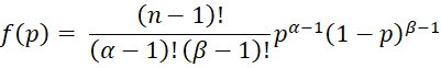
This is a special case of the pdf of the beta distribution where the parameters don’t have to be positive integers.
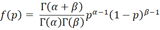
Figure 1 shows key properties of the beta distribution.

Figure 1 – Key properties of beta distribution
When we use the beta distribution as our prior distribution, then the specific values of the α and β parameters determine how our prior beliefs correspond to a prior sample (even when no such sample was made) with α successes and β failures in n = α + β trials. If we believe that the probability of success and failure are about equal (and so the distribution is symmetric with α = β), then the mean is .5. If α < β then the distribution is skewed to the right (skewness is positive), while if α > β then the distribution is skewed to the left (skewness is negative). Also, the higher the value of n = α + β, the smaller the variance, and so the more confident we are of our prior beliefs.
Figure 2 contains plots of the beta distribution based on different values of α and β.
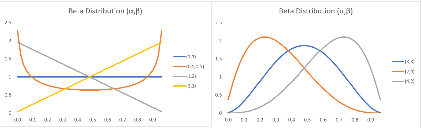
Figure 2 – Beta distributions
Non-informative Priors
Notice too that if α = β = 1, then the beta distribution, Bet(1, 1), is equivalent to the uniform distribution on the interval (0, 1). We can use the uniform distribution as a non-informative prior, where we have no prior belief as to the probability of success (i.e. getting heads when tossing a coin) and so all outcomes are equal.
If our prior belief is that heads and tails are equally likely we can use a prior distribution of Bet(1,1), but if we are more certain of this we can use a prior distribution of Bet(3,3), Bet(10,10) or even higher, depending on our level of certainty. If we are less certain, then we can use a prior distribution of Bet(.5, .5), also called Jeffreys prior. All of these are considered to be non-informative priors.
If instead, we believe that on average, heads occur 3 times as often as tails, then we can use a Bet(3,1) prior distribution. If we are more confident of this belief, we can use a Bet(6,2), Bet(30,10) or even a higher beta distribution. In general, we can choose the value of α = nμ or α = (n–2)mode+1 (for n > 2) and β = n – α.
Property
Property 1: If x is the number of successes in n trials, following a binomial distribution with unknown parameter p, and the prior distribution is Bet(α, β) then the posterior distribution is p|x ∼ Bet(α′, β′) where
α′ = α + x β′ = β + n – x
Proof:
![]()
Thus
![]()
![]()
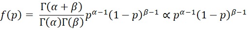
Since f(p|x) is proportional to the pdf of Bet(α′, β′), this completes the proof.
Weighted Average
By Property 1, where m = α + β, the expected posterior is

![]()
![]()
This means that the expected posterior is the weighted average of the expected prior and the sample mean. If we consider m as the pseudo-sample size of the prior, then weights for the expected prior and sample mean are based on the sample sizes of the prior and the data.
Simple Example
Example 1: Suppose that we use a uniform prior distribution and a recent poll of 100 people shows that 55 people favor Alan and 45 favor Bill, estimate the posterior distribution. What is the probability that Alan will win?
Based on Property 1, we see that the posterior distribution p|x ∼ Bet(1+55, 1+45) = Bet(56, 46). Therefore, we conclude that the probability that Alan will win is 1-BETA.DIST(.5,56,46,TRUE) = 84%.
Treatment Effectiveness
Example 2: In a trial of a new drug to prevent patients having a rare viral infection, 200 people at random were given the drug and 200 were not given the drug. After exposure to the virus, 4 people in the control group came down with the virus, while none in the treatment group got the virus. Determine whether the treatment is effective.
We can view this problem as 4 tosses of a coin (the 4 people who contacted the virus) where heads is that the person is in the control group and tails is the person is in the treatment group. This can be modelled using a binomial distribution.
Frequentist approach
Using the frequentist approach, let p = the probability that the person comes from the control group. The null hypothesis is that p ≥ .5. We note that BINOM.DIST(0,4,.5,TRUE) = .54 = .0625. Since this value is larger than alpha = .05, we cannot reject the null hypothesis that no treatment is better than the drug.
Bayesian approach
Using the Bayesian approach, we decide to use a uniform prior, i.e. p ~ Uniform(0,1) = Bet(1,1) since we have no strong beliefs and so any probability between 0 and 1 seems equally likely. After the trial, however, based on Property 1, the posterior distribution is p|x ~ Bet(1+4,1+4-4) = Bet(5,1).
Now the mean of the Bet(α,β) distribution is α/(α+β), and so the mean probability that a virus infected person comes from the control group is 5/6. Thus, the probability that a virus infected person comes from the treatment group is 1-5/6 = 1/6. Since 5/6 > 1/6, the evidence and our prior beliefs points in the direction of the effectiveness of the drug.
In fact, the probability that p ≥ .5, indicating that the drug is at least as effective as no drug is
1-BETA.DIST(.5,5,1,TRUE) = 96.9%
Note too that the variance of a beta distribution Bet(α,β) is αβ/[(α+β)2(α+β+1)]. Thus, prior to the collection of data the standard deviation of p is .29 (namely 1 divided by the square root of 3⋅4). After the collection of data the standard deviation is reduced to .14 (namely the square root of 5/(36⋅7)).
Examples Workbook
Click here to download the Excel workbook with the examples described on this webpage.
References
Gelman, A., Carlin, J. B., Stern, H. S., Dunson, D. B., Vehtari, A., Rubin, D. B. (2014) Bayesian data analysis, 3rd Ed. CRC Press
https://statisticalsupportandresearch.files.wordpress.com/2017/11/bayesian_data_analysis.pdf
Hoff, P. D. (2009) A first course in Bayesian statistical methods. Springer
https://esl.hohoweiya.xyz/references/A_First_Course_in_Bayesian_Statistical_Methods.pdf
Reich, B. J., Ghosh, S. K. (2019) Bayesian statistics methods. CRC Press