Objective
We illustrate how to perform hypothesis testing for binomially distributed data using a Bayesian approach. See Bayesian Hypothesis Testing for background information.
Two-sided Example
Example 1: We want to determine whether a coin is fair and so we test the following null and alternative hypotheses where p = the probability that the coin will produce heads.
H0: p = .5 (fair coin)
H1: p ≠ .5
We then toss the coin 100 times and get 60 heads. Evaluate whether the coin is fair based on the data using a uniform prior.
Basic Concepts
Here, the null hypothesis takes one value and so we can use the prior f(p) = 1 for p = .5 and f(p) = 0 elsewhere. For the alternative hypothesis, p can take any value in the interval [0, 1] except p = .5 (although this exception doesn’t impact the integral in the following expression). Thus, for any data X, the Bayes Factor is
We, of course will assume that the data follows a binomial distribution and the prior for H1 follows a beta distribution. Initially we assume that the prior is the uniform distribution on [0, 1], which is equivalent to the Bet(1,1) distribution. This corresponds to our having no preconceived notion about the value of p if the alternative hypothesis is true.
Example 1 (Continued)
Using the above concepts
P(x = 60|H0) = BINOM.DIST(60,100,.5,FALSE) = .010844
P(x = 60|H1) is specified by
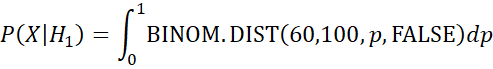
In general, we use the following formula where s = the # of successes in n trials and alpha and beta are the parameters of the beta prior. We can evaluate this integral using the Real Statistics INTEGRAL function and calculate the Bayes factor BF10 as described in Figure 1.
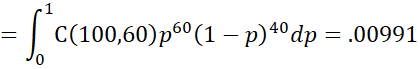
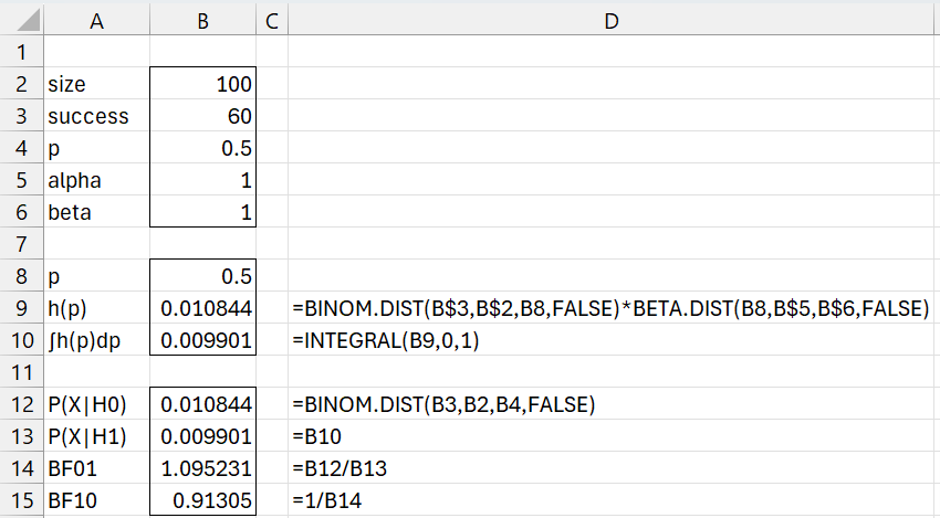
Figure 1 – Bayesian binomial test
We see from cell B15 that
![]()
which means that the evidence slightly favors the null hypothesis.
If instead the prior is Bet(4,2), we obtain
![]()
This is calculated by changing the values of alpha and beta in cells B5 and B6.
If the prior is Bet(2,4), we get
![]()
If our original test value for p is .4 with a uniform prior then since
P(x = 60|H0) = BINOM.DIST(60,100,.4,FALSE) = .000024425
we obtain
![]()
If also the prior is Bet(4,2), then
![]()
Finally, if our original test value for p is .6 with a uniform prior then
![]()
One-sided Example
Example 2: Calculate the Bayes Factor for the following hypotheses based on the same data as in Example 1.
H0: p = .5 (fair coin)
H+: p > .5
Using the uniform prior we obtain the following approximation for BF+0. First, we calculate
q = (1-BINOM.DIST(60,100,.5,TRUE))+BINOM.DIST(40,100,.5,TRUE) = .046044
Then, we can approximate the Bayesian factor as follows
BF+0 = (2 – q)BF10 = (2 -.046044)(.91301) = 1.784059
If instead the alternative hypothesis is
H–: p < .5
then
BF0- = qBF10 = (.046044)(.91301) = .042041
This approximation is valid provided p = .5 and alpha = beta = 1.
Examples Workbook
Click here to download the Excel workbook with the examples described on this webpage.
References
Wikipedia (2025) Bayes factor
https://en.wikipedia.org/wiki/Bayes_factor
Nicenboim, Schad, D. J., Vasishth, S. (2025) Bayes factors. Introduction to Bayesian Data Analysis for Cognitive Science
https://bruno.nicenboim.me/bayescogsci/ch-bf.html