Objective
Describes the Bayesian version of the non-parametric Signed-Ranks Test. This test is typically used when the assumptions for the one-sample or paired t-test is not met.
Basic Concepts
Suppose that you have a sample Z = z1, …, zn and want to test the hypotheses
H0: μ > μ0
H1: μ ≤ μ0
where μ is the mean of the population from where Z came from and μ0 is some constant (usually zero). The classical non-parametric test is the Wilcoxon Signed Ranks test. We now present a Bayesian approach to this test.
This approach also covers the paired sample version where you have two paired samples X = x1, …, xn and Y = y1, …, yn, and want to test the hypotheses
H0: μX > μY
H1: μX ≤ μY
This test is equivalent to the one sample case where μ is the mean of the population from which the sample Z = z1, …, zn came from where zi = yi – xi.
Example
Example 1: Perform the Bayesian Signed Ranks test for the paired data in columns A and B of Figure 1.
We first calculate T+ as shown on the right side of Figure 1.
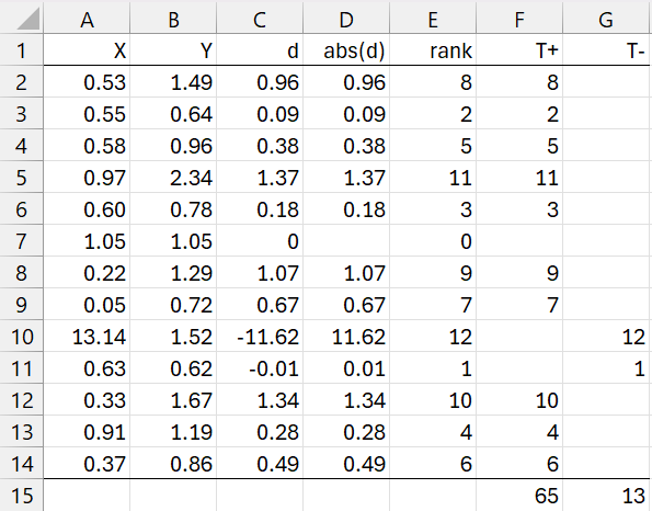
Figure 1 – Calculation of T+ and T–
As usual, we first calculate the differences as shown in column C. Here cell C2 contains the formula =B2-A2. We now ignore any zero differences, reducing our sample size from 13 to 12 since cell C7 contains a zero value. Column D contains the absolute values of the elements in column C, and column E provides the ranks of these values. E.g. cell E2 contains the formula =IF(C2=0,0,RANK.AVG(D2,D$2:D$14,1)). Column F contains the ranks corresponding to positive elements in column C and column G contains the ranks corresponding to negative elements in column C. Thus, cell F2 contains the formula =IF(C2>0,E2,””) and G2 contains =IF(C2<0,E2,””).
Finally, we calculate T+ = 65 (cell F15) as the sum of the elements in columns F and T– = 13 as the sum of the elements in column G. Since T+ + T– = C(n+1,2) = n(n+1)/2, once you know T+, the value of T– is determined. For this example, n(n+1)/2 = 12(13)/2 = 78, and so T– = 78 – 65 = 13, as expected. Thus, we only need to deal with T+.
We also define n+ to be the number of elements in column F and n– to be the number of elements in column G, where clearly n+ + n– = n. For Example 1, n+ = 10 and n– = 2. We also define p = n+/n.
Bayesian approach
For the Bayesian approach to the test, we consider the parameter φ, which is the population version of p. φ takes values between 0 and 1. For n ≥ 6, we can create a discrete approximation to the distribution of φ using a grid approach (see Bayesian Grid Approximation).
For any value of between 0 and 1, we randomly assign a + or – to the integers 1 through n so that the probability of a + is φ. We then calculate the value of T+ as was done in Figure 1. We do this a large number of times, say N = 30,000, and estimate the likelihood by the proportion of such samples whose T+ value is the same as the original sample’s T+ value (65 for Example 1).
For example, if φ = .75, then for Example 1, the first 15 of 30,000 iterations are as shown in Figure 2.
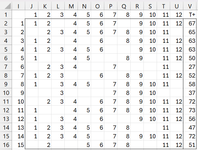
Figure 2 – Creating grid entries
Here row 1 contains the 12 possible ranks and column I corresponds to the iterations (15 out of 30,000 shown). The cells with values in the range J2:U30001 correspond to positive values and the blank cells correspond to negative values. These results are obtained by placing the formula =IF(RAND()<=0.75,J$1,””) in cell J2, highlighting range J2:U30001, and pressing Ctrl-R and Ctrl-D.
Next, we calculate the T+ values for each iteration in column V by placing the formula =SUM(J2:U2) in cell V2, highlighting range V2:V30001, and pressing Ctrl-D. We see that of the first 15 T+ values in column V, only the second one matches the value, 65, calculated in Figure 1.
From the data in column V, we can estimate the “distribution” value at φ = .75 via the formula =COUNTIF(V2:V30001,65)/30000, which turns out to be 915/30000 = .0305.
Note that if there are ties in column C of Figure 1, then the rank values will be different from those that appear in row 1 of Figure 2.
Creating the grid
To obtain the distribution, we perform the above approach for 200 values of φ, namely the values .0025 + .005(i–1) for i = 1, 2, …, 200. This is done by placing 1 in cell X2 and .0025 in cell Y2, the formulas =X2+1 in cell X3 and =Y2+.005 in cell Y3, highlighting range X3:Y201, and pressing Ctrl-D.
The elements in column Z implement the sampling approach described above for each φ, producing the likelihood values. This can also be done by inserting the formula =BayesSR1(E$2:E$14,F$15,Y3) in cell Z2, highlighting the range Z2:Z201, and pressing Ctrl-D. This function is explained in Bayesian Signed Ranks Test Support.
We add up all the values in column Z to obtain 2.047 (cell Z202). We then divide each value in column Z to obtain the pdf f(φ) values in column AA. Finally, we estimate the cdf F(φ) values in column AB by placing the formula =AA2 in cell AB2, =AA3+AB2 in cell AB3, highlighting range AB3:AB201, and then pressing Ctrl-D.
Figure 3 displays some of the 200 rows from the output.
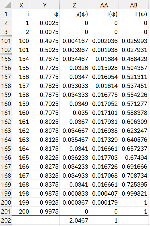
Figure 3 – Discrete grid estimation
The prior distribution for φ is the uniform distribution, where f(φi) = 1/200.
We now use the approach described in Bayesian Analysis using Grids to produce the output shown in Figure 4. In particular, we insert the following formula
=GridDesc(Y2:Y201,AA2:AA201,TRUE,0.5)
in range AH2:AI12.
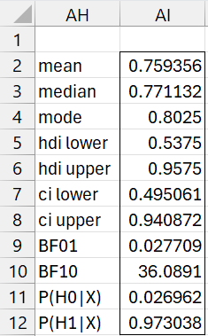
Figure 4 – Bayesian analysis
From the output, we see that the Signed Ranks Tests favors the alternative hypothesis by about 36 to 1, with the probability that the alternative hypothesis is true at 97.3%.
Large Sample Approximation
For n > 24, the posterior distribution of φ can be approximated by the beta distribution Bet(a, b) where a = a0 + a1 and b = b0 + b1, for a prior distribution of Bet(a0, b0) with
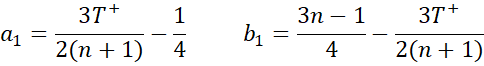
Even though the sample size of n = 12 for the data in Figure 1 is well below 24, we now repeat the analysis for Example 1 using the large sample approximation. The results are as shown in Figure 5 using the array formula =BayesBeta(AM6,AM7,TRUE) in range AQ2:AR14.
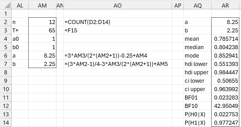
Figure 5 – Bayesian analysis (large sample)
Despite the fact that the sample size is much smaller than the recommendation, the large sample approach yields reasonably similar results to that obtained via the small sample approach.
Worksheet Functions and Data Analysis Tool
Starting with Rel 9.5, the Real Statistics Resource Pack will provide various Excel capabilities that implements the Bayesian Signed Ranks Test.
Click here for details.
Examples Workbook
Click here to download the Excel workbook with the examples described on this webpage.
References
Kruschke, J. K. (2015) Doing Bayesian data analysis. 2nd Ed. Elsevier
https://sites.google.com/site/doingbayesiandataanalysis/
Chechile, R. A., Barch, D. H. Jr. (2025) Distribution-free Bayesian analyses with the DFBA statistical package
https://link.springer.com/article/10.3758/s13428-025-02605-6