We now describe the structural model for repeated measures ANOVA where there are two within-subjects factors.
Definitions
Definition 1: We modify the structural model of Definition 1 of Two Factor ANOVA with Replication as follows. Note that we will use a to indicate the number of levels for factor A (instead of r) and b to indicate the number of levels for factor B (instead of c). Also, m = the number of subjects or participants.
We use terms such as x̄i (or x̄i.) as an abbreviation for the mean of {xijk: 1 ≤ j ≤ b, 1 ≤ k ≤ m}. We also use terms such as x̄j (or x̄.j) as an abbreviation for the mean of {xijk: 1 ≤ i ≤ a, 1 ≤ k ≤ m}.
We define the effects αi and βj where
![]()
Similarly, we define ai and bj where
![]()
We use δij for the effect of level i of factor A with level j of factor B, i.e. the interaction of level i of factor A and level j of factor B. Thus, δij = μij – μi – μj + μ. Similarly, we have
![]()
It is easy to show that
![]()
Finally, we can represent each element in the sample as
![]()
where εijk denotes the error (or unexplained) amount, where
![]()
and γk is a random effect corresponding to the subjects/participants. All the interaction terms, i.e. (αγ)ik, (αβ)jk, and (αβγ)ijk, are also random effects; together they make up the error components of our model.
As before we have the sample version
![]()
where eijk is the counterpart to εijk in the sample. The null hypotheses for main effects are:
H0: µ1. = µ2. = ··· µa.(Factor A)
H0: µ.1 = µ.2 = ··· µ.b(Factor B)
These are equivalent to:
H0: αi = 0 for all i (Factor A)
H0: βj = 0 for all j (Factor B)
In addition, there is a null hypothesis for the effects due to the interaction between factors A and B.
H0: δij = 0 for all i, j
Definition 2: Using the terminology from Definition 1 of Two Factor ANOVA with Replication, except that we use a for the number of levels in factor A (instead of r) and b for the number of levels in factor B (instead of c), and also adding C = the participant factor and m = number of participants, define:
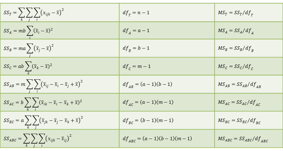
We can also define four types of between-group terms.
![]()
And similarly for BetAC and BetBC. There is also the following BetABC version:
![]()
![]()
![]()
Properties
Property 1:
![]()
![]()
Proof: It is clear that
![]()
![]()
If we square both sides of the equation, sum over i, j, and k and then simplify (with various terms equal to zero as in the proof of Property 2 of Basic Concepts of ANOVA), we get the first result. The second result is trivial.
Property 2: If a sample is made as described in Definition 1 of Basic Concepts of ANOVA, with the xijk independently and normally distributed and with all 

![]()
![]()
Proof: The proof is similar to that of Property 1 of Basic Concepts of ANOVA.
Theorem 1: Suppose a sample is made as described in Definitions 1 and 2 of Two Factor ANOVA with Replication, with the xijk independently and normally distributed.
If all μi are equal and all 
![]()
If all μj are equal and all 
![]()
Also, under certain circumstances,
![]()
Proof: The result follows from Properties 1 and 3 of F Distribution.
Property 3:
![]()
![]()
![]()
![]()
We use the following tests:
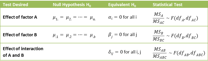
If the null hypothesis for factor A is true, then 
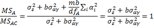
whereas if the null hypothesis is not true then 
Reference
Howell, D. C. (2010) Statistical methods for psychology (7th ed.). Wadsworth, Cengage Learning.
https://labs.la.utexas.edu/gilden/files/2016/05/Statistics-Text.pdf