We show how to perform Repeated Measures ANOVA where there are two within-subjects factors.
Principal Example
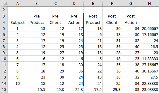
Example 1: A company has created a new training program for their customer service staff. To test the effectiveness of the program they took a sample of 10 employees and assessed their performance in three areas: Product (knowledge of the company’s products and services), Client (their ability to relate to the customer with politeness and empathy), and Action (their ability to take action to help the customer). They then had the same 10 employees take the training course and rated their performance after the program in the same three areas. Based on the data in Figure 1, determine whether the program was effective.
Figure 1 – Data for Example 1
There are two treatment factors: Training (with levels pre and post) and Skill (with levels Product, Client, and Action) plus the Subject factor. We begin by creating the worksheet in Figure 2.
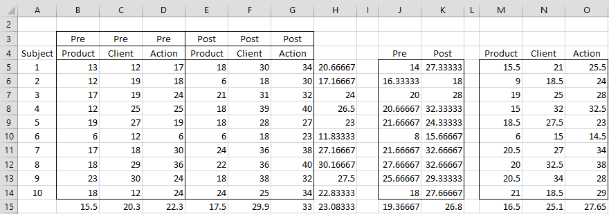
Figure 2 – Data for Example 1 plus treatment means
In addition to the raw data (range A3:G14), Figure 2 shows the means for the interaction between the various factors: Training × Skill (B15:G15), Training × Subject (J5:K14), Skill × Subject (M5:O14), as well as the means for each factor: Training (J15:K15), Skill (M15:O15) and Subject (H5:H14). Finally, the grand mean is shown in cell H15.
Analysis
In what follows we use a to indicate the number of levels for factor A and b to indicate the number of levels for factor B. Also, m = the number of subjects or participants in each level of A × B, and n = the total number of subjects. Thus n = m ⋅ a ⋅ b.
We will test the null hypotheses:
H0: µ1. = µ2. = ··· µa. (Factor A)
H0: µ.1 = µ.2 = ··· µ.b (Factor B)
H0: δij = 0 for all i, j (Interaction)
See Two Within-subjects Factors Structural Model for definitions of these terms and more details about the structural model being used.
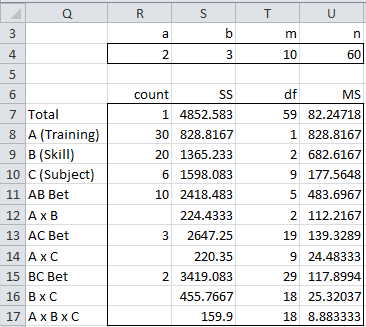
From the information in Figure 2, we create the tables in Figure 3.
Figure 3 – Construction of ANOVA for Example 1
Row 4 contains the values of a, b, m, and n for Example 1. E.g. a = the number of Training levels = COUNTA(J3:K3) and n = PRODUCT(R4:T4) or COUNT(B5:G14). The various degrees of freedom are calculated from these values as described in Definition 2 of Two Within-subjects Factors Structural Model. Figure 4 displays some representative formulas.
Figure 4 – Representative df from Figure 3
The count values in column R are used to calculate the SS values in column S. In all cases, the count value equals . The values for SS are calculated as in Definition 2 of Two Within-subjects Factors Structural Model. Some examples are given in Figure 5.
Figure 5 – Representative SS from Figure 3
Output
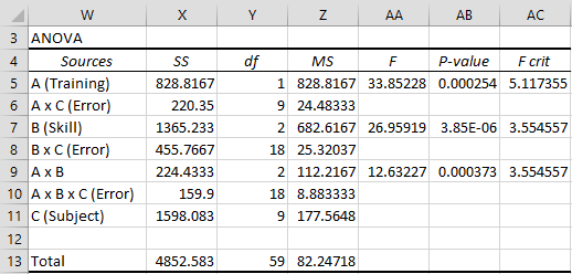
From the table in Figure 3, we arrive directly at the ANOVA analysis in Figure 6.
Figure 6 – ANOVA with repeated measures
Sphericity
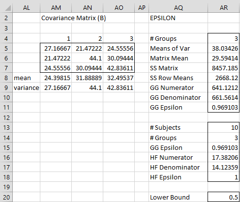
Note that the p-values for both main effects and the interaction effect are significant, but before we conclude this definitively we need to take sphericity into account. For the Training factor, there are only two levels, and so sphericity is automatic. Since the Skill factor has more than two levels we need to calculate the GG and HF epsilon correction factors (see Figure 7) as we did in Sphericity for the one within-subjects factor analysis.
Figure 7 – Calculation of sphericity corrections for Skill (B) effect
Here the covariance matrix is calculated using the array formula =COV(M5:O14). We see that GG epsilon is close to 1 and HF epsilon is 1, and so it appears that there is no problem with sphericity.
We also need to worry about the sphericity of the interaction effect. For this we will simply look at the lower bound which for the interaction effect is equal to =
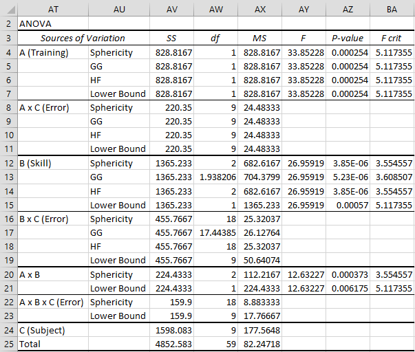
= .5. Figure 8 provides a revised version of Figure 6 taking sphericity into account.
Figure 8 – Revised ANOVA with repeated measures
We see from Figure 8 that the main effects and interaction effects are all significant. We now use planned and/or unplanned tests to better understand what is going on.
Contrasts
As described in ANOVA with Repeated Measures with One Within Subjects Factor where the sphericity assumption holds we can use the same types of tests that we used for ANOVA with independent variables. For these tests the standard error is based on MSE where the appropriate value of MSE is employed: MSA×C with dfA×C = (a–1)(m–1) for the main effect A, MSB×C with dfB×C = (b–1)(m–1) for the main effect B and MSA×B×C with dfA×B×C = (a–1)(b–1)(m–1) for the interaction effect A × B.
Where sphericity doesn’t hold it is best to use the contrast-specific standard error and not use an MSE type value. In fact, it is probably better to use the contrast/specific standard error in all cases. Unplanned tests can also be used as described in ANOVA with Repeated Measures with One Within Subjects Factor.
Basic example
Example 2: For the data in Example 1 determine whether there is a significant difference in the training program for each of the three skills.
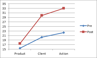
Figure 9 – Comparison of means for interaction
As we can see from Figure 9, it appears that training improves performance for each skill, although only slightly in the case of the Product skill. We need to determine whether any of these differences are significant. We do this by performing pairwise comparisons.
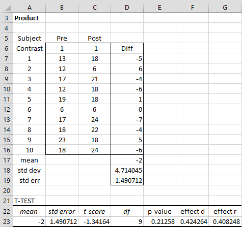
Figure 10 – Contrast for pre and post-training for Product
The test for the Product skill in Figure 10 shows there is no significant difference between the means for Product pre-test and post-test (p > .05). If we perform the same analysis for Client we see there is a significant difference: t(9) = -4.63, p = .001 < .05, d = 1.47. Similarly for Action: t(9) = -11.21, p = 3E-05 < .05, d = 2.43. Note that the contrast analysis is equivalent to the t-test on paired samples. Even if we use a Bonferroni or Dunn-Sidák correction, the results will be similar.
If we had chosen to make the 6 unplanned tests using Tukey’s HSD, including a test of Product pre-training vs. post-training, then from the above analysis we know that tobs = -1.34. We need to compare the absolute value of this observed value of t with the critical value of t (as described in Unplanned Comparisons for ANOVA).
First, we look up the q critical value q(k, df, α) where α = .05, k = ab = 6, and df = m – 1 = 9. From the Studentized Range q Table, we have q(6, 9, .05) = 5.024, and so tcrit = = 3.55. Since |tobs| = 1.34 < tcrit = 3.55 we conclude that there is no significant difference between the Product performance before and after the training.
More complicated example
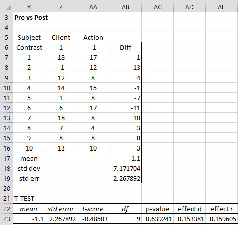
Example 3: For the data in Example 1 determine whether the training has had the same effect on the Action skill as it has had on the Client skill.
We test the following null hypothesis:
H0: μAction×Post – μAction×Pre = μClient×Post – μClient×Pre
We now compare the differences between Post and Pre-training for Action with the differences Post and Pre-training for Client.
Figure 11 – Contrast for Training effect on Client vs Action
Here we see that p = .64 > .05 = α, and so we conclude there is no significant difference between the training effect on Client skills vs. Action skills.
Data Analysis Tools
The Real Statistics Resource Pack provides the Two-way Repeated Measures Anova tool that can provide the analysis described above. The One Factor Repeated Measures Anova tool can be used to obtain contrast analyses.
Click here for more information about these data analysis tools and how to use them.
Examples Workbook
Click here to download the Excel workbook with the examples described on this webpage.
Reference
Howell, D. C. (2010) Statistical methods for psychology (7th ed.). Wadsworth, Cengage Learning.
https://labs.la.utexas.edu/gilden/files/2016/05/Statistics-Text.pdf


Hi Charles,
I have a similar situation as the one in the example above, but with two between subjects factors (with 4 levels). I have a pre-test and post test with ten items, where 5 items test one construct and 5 items test a different construct. I also want to compare total scores out of 10. But I have a control group and three test groups. I feel like I am peeling an onion trying to figure out which anova or manova to run. Oh, and the samples are unbalanced. It seems like the easiest thing would be to compare the difference scores between post and pre via regression. Any tips?
Data looks something like this:
PRE POST
Part 1 Score Part 2 Score Total Part 1 Score Part 2 Score Total CONTROL
TEST GROUP 1
TEST GROUP 2
TEST GROUP 3
Sorry, the format did not post properly.
PRE PRE PRE POST POST POST
Part I Part II Total Part I Part II Total
Control
Test Group 1
Test Group 2
Test Group 3
*correction: I have two within (pre and post/part 1, part 2 and total scores) and one between subjects factor (treatment group).
Hello Mike,
If I understand correctly, you have an unbalanced repeated measures ANOVA with two within-subjects factors and one between-subjects factor. You will have many challenges with this sort of design, including:
– how to interpret the results
– how to test the assumptions
– how to correct for sphericity
Real Statistics handles unbalanced repeated measures ANOVA with one within-subjects factor and one between-subjects factor. See
https://real-statistics.com/anova-repeated-measures/one-between-subjects-factor-and-one-within-subjects-factor/
https://real-statistics.com/anova-repeated-measures/repeated-measures-anova-using-regression/mixed-repeated-measures-anova-using-regression/
You can modify the approach described on the above webpages to handle the second between-subjects factor, although handling sphericity will probably be a challenge.
In any case, it seems that your sample is not very large and so this complicated approach is probably overkill since the power of the test will likely be low. I would focus on the hypotheses that you really need to test and see whether you can come up with a simpler design tailored to accomplish this.
Charles
Thank you very much for the reply! It is very helpful!
You understood correctly (or, rather, I seem to have managed to explain it in an comprehensible way). And since I have already been referring to the pages you suggest, I think I am on the right track: definitely ANOVA via regression and I definitely need to try to simplify, at least if I am going to do it on my own.
I already have the data, so I cannot change the experimental design or research questions, but perhaps I can change how I want to answer the questions.
Sample size is <30 for each of the four groups.
Below are the possibilities I have come up with at this point. would you recommend any of these over the others?
1) Similar studies in my field have run multiple single factor ANOVAS to compare mean scores across treatment groups on pretest and posttest, separately. (I would need to run a third analysis on the composite score.) If they find no difference between groups in pretest means, but a difference between groups in posttest means, they conclude that treatment(s) had an effect. But if I did it this way I would want to at least do a Bonferroni correction, and I do not think all the studies I have read have done so…
2) I could make the analysis a bit more robust by running three one factor ANOVAS to compare difference scores on part 1, part 2, and cumulative, separately. Again with Bonferroni correction.
3) I have also considered a two-factor ANOVA on difference scores to compare mean differences on part 1 and part 2 of the test across treatment groups. (Advantage here is that I have a better idea of a difference in performance between part 1 and part 2.) Then I could run a one factor analysis to compare difference scores on the sum of the two parts. Since the total score is just a sum of part 1 and part 2, I should be treating this separately anyways. Also here with Bonferroni correction.
4) Finally, I could do three repeated measures ANOVAS on before/after means on Part1, Part2 and Total separately. Again with Bonferroni.
Do any of these seem more robust to you than the others?
Thanks again! I have not referred to your site in a while, but I have been using your add in for several years. I have made reference to it in a couple papers and presentations as well. This is truly a great resource for so many people!
Hi Mike,
If you are only interested in the differences, then you should focus on these. In this case, you can even run a single ANOVA and avoid Bonferroni. Then when you do the post-hoc analysis you can use Tukey’s HSD.
Charles
If I run one two-way ANOVA on the difference scores across the four groups, then I should exclude the total score from the analysis, since it is merely a sum of part I and part II, and would already be implicitly included in the comparison of rows, right?
Mike,
If the total can be calculated as a linear combination of the values from the other groups, then you should exclude it from the analysis.
Charles
Thank you!
Dear Charles,
Thank you for your very useful tutorial and great website! I have a question regarding the epsilon factor for the interaction term. Do you know if it’s possible to compute the Greenhouse-Geisser correction factor for the interaction, instead of using the lower bound? (The latter being, as I understand it, too conservative).
Many thanks,
Best – Raphael
Hello Raphael,
I imagine that it is possible, but I haven’t found the correct formulas. If you do find out how to do this, please let me know.
Charles
Charles,
The last paragraph in this section does not make sense to me. Examples 2 and 3 are to determine the effect of the program (ie, comparison pre vs post). The two data ranges to be selected as input contain only average values of individual subjects for each factor of interest. To perform the comparison, the difference between pre and post values should be used as input data.
-Sun
Charles,
I have 2 questions for you:
1. Under Figure 7, you stated that “GG epsilon is close to 1 and HF epsilon is 1, so it appears that there is no problem with sphericity.” I am not sure I understood this one correctly. Do you mean if the GG epsilon or HF epsilon value is close to 1, then the data meet the sphericity assumption?
Based on the covariance matrix for the factor B, it is clear that it does not have the compound symmetry form. Therefore, I’d think that the factor B does not meet the sphericity assumption. Please clarity the statement above.
2. In Figure 8, it is not clear what sub-individual rows within each factor mean (ie, sphericity, GG, HF, and low bound) and how their SSs have been calculated. I thought the sphericity correction can be made on the degree of freedom. But, it seems that further correction can be made on the data values as well. Your step-by-step explanation on what individual sub-rows mean and how corresponding SS can be calculated.
Thanks,
-Sun
Charles,
In the second from the last paragraph in this section, it referenced to Figure 5 in the Sphericity section. But, there is no Figure 5 in that section. Please update the text to reflect the correct reference.
Thanks,
-Sun
Hello Sun,
Thanks for identifying this error. I have not corrected this on the webpage, specifying the correct link. Unfortunately, I am currently unable to create an automatic link to the correct webpage. I will do this at a later time. As always, thanks for your diligence in finding mistakes on the website.
Charles
Hi Charles,
how would you test the interaction between A and Subject (C). In my data A is not significant but I suspect the interaction between subject and A is significant, that is, the effect of A is evident for some subjects, not others. Is that possible? Thanks, best regards
Fabrizio,
AxC interaction is generally not of much interest since there is normally variation based on the subject. Why is this interaction of interest to you. AxB is generally of interest. This webpage describes how to test the significance of this interaction.
Charles
Hi Charles,
thank you very much for your quick answer. Let me briefly explain: For each subject, I have 10 measurements “Pre”and 10 measurements “Post”. I expect to be a drop in the value between Pre and Post, but I do know how to test it. If I perform a t-test between Pre and Post for each subject, I get a very significant P-values (after Bonferroni correction), but somehow I believe the t test is not appropriate within subjects. Any idea? Thanks, best regards.
Fabrizio,
The approach depends on what hypothesis you are trying to test. If you want to test whether there is a significant difference between Pre and the last Post (across all the subjects), then you can use a paired t test. If you want to determine whether there is a significant difference between other of the Post measurements (either with Pre or between two of the Post), then you can use Contrasts with a Bonferroni correction. See Figure 3 on https://real-statistics.com/anova-repeated-measures/one-within-subjects-factor/.
You can also perform more elaborate tests (e.g. Pre vs the average of the Post) by using Contrasts, as explained in Figure 3.
You can also perform Tukey’s HSD, as described at the end of the above referenced webpage.
Note that in all of these tests, you are making comparisons across all the subjects (not one subject at a time).
All these tests can be performed using the Real Statistics One Repeated Measures ANOVA data analysis tool.
Charles
How do you calculate the sum of squares for AC Bet, A x C, BC Bet, B x C, please?
Ryan,
Figure 4 shows the formulas for AB Bet and A x B. To get AC Bet just substitute the B values in the formula for AB Bet by the C values. To get A x C just substitute the B values in the formula for A X B by the C values. For BC Bet and B x C you need to substitute the A values by the C values.
Charles
Hi Charles,
How to calculate SS for C only?
Thanks,
Sarah
Hi Sarah,
Thanks for your question. To make things clearer, I have just added this information to the webpage.
Charles
Thanks a lot for your nice stats explanation and useful tool.
I have the following data and I need to find the difference between (old and young), (young and kid) and (kid and young).
Would it be possible that you could please help me?
here is my data:
subjects measures conds values
1 weight old 71
2 weight old 64
3 weight old 79
1 height old 172
2 height old 151
3 height old 179
1 heartbeats old 72
2 heartbeats old 99
3 heartbeats old 90
1 weight young 84
2 weight young 83
3 weight young 59
1 height young 161
2 height young 176
3 height young 198
1 heartbeats young 80
2 heartbeats young 79
3 heartbeats young 62
1 weight kid 23
2 weight kid 25
3 weight kid 30
1 height kid 146
2 height kid 98
3 height kid 58
1 heartbeats kid 68
2 heartbeats kid 86
3 heartbeats kid 84
Based on the type of data you have presented it seems like you have two dependent variables, namely weight and heartbeat and one independent variable age group (kid, young, old). This is compatible with MANOVA. See MANOVA for more details.
Whether this is really the test to use depends on the hypotheses you want to test.
Charles
I’m having some trouble filling out the dialog box, and I’m not sure how arrange the rows and columns in excel. How is a two factor x two level RM ANOVA different from a one-factor four level RM ANOVA in the column and row layout?
My ANOVA table always has missing cells that do not calculate. I’m running iOS 10.11.1 (El Capitan) and Excel 2011 for Mac.
Michael,
The Real Statistics Resource Pack doesn’t currently support a two within subjects factor RM ANOVA. It does support a mixed factor RM ANOVA. The layout of the data for this model is as described in Figure 19 of the following webpage:
https://real-statistics.com/anova-repeated-measures/one-between-subjects-factor-and-one-within-subjects-factor/
The data layout for a one factor RM ANOVA model is described in Figure 5 of the following webpage:
https://real-statistics.com/anova-repeated-measures/sphericity/
The versions of the algorithms used require balanced models with no missing data. I expect to allow for unbalanced models with missing data in one of the next two releases of the software.
Charles
Hi. Your work is excellent, but I’d appreciate some help. I can’t find the menu entry for ‘two-way anova with repeated measures on both factors’. It’s there in the multivariate workbook , but not on my computer. When I look at the RealStatistics menu in Excel I see ‘Analysis of Variance’; when I click on that I’m offered Anova:one factor, Anova:two factors, Anova:three fixed factors, Manova single factor, Nested anova:two factors, Repeated measures:one factor, Repeated measures: mixed, and Ancova. None of those seem to be what I want.
I’ve had the same problem on both the Windows version and the Mac version. I’m sure I’m missing something! If you could tell me where to find the right button I’d be very grateful.
Best wishes and thank you in advance
Thomas Green
Sorry Thomas, but I don’t yet provide a two-way anova with repeated measures on both factors option.
Charles
Aieee! There’s one in the Workbook, or am I mistaken? It’s exactly my design – each participant did the same 3 programming problems (factor 1) with or without syntax highlighting (factor 2). I could pool the scores over problems to get a simple test of the effect of highlighting, but the graphs suggest an interaction effect – syntax highlighting seems to be more useful on the harder problems, as you’d expect. What’s my best route forward – planned comparisons? It’s a bit cheeky of me to ask for stats advice, when you’ve already put in so much unpaid work just for the benefit of total strangers. Please feel free to ignore me if you like.
Many thanks,
Thomas
Thomas,
Yes, there is an example of your design described on the website, and you can indeed find the example in the Examples Workbook. I just haven’t implemented it yet in the software. You can use planned comparisons to pinpoint the effect. I give quite a few examples (plus support in the Real Statistics Resource Pack) of how to do this for two factor ANOVA (but not for repeated measures) and one factor ANOVA with repeated measures.
Charles
hai charles,
how about if my study is just two-way within subjects?? what do you think are its assumptions???
thank you 🙂
What do you mean by “how about if my study is just two-way within subjects??” How does your study differ from the type of analysis described on the referenced webpage?
The assumptions for Anova with repeated measures (in general) are:
– Dependent variables have intevral measure
– Independent variables should be repeated measure
– No significant outliers
– Distribution of each group should be normal (although the test is pretty robust to violations of this assumption)
– Sphericity (although the correction factors can be used when this assumption is violated).
Charles
Also, I see from your site you can adapt a two-way ANOVA with repeated measures on only one factor for an “Unbalanced model”. Can you do the same here for a two-way ANOVA with repeated measures on both factors?
David,
I have not yet worked on using regression approaches (or general linear models) for this situation. I plan to turn my attention to this situation shortly.
Charles
I’ve installed the Resource Pack for Excel 2007. Is the “Repeated Measures ANOVA” function in the 2007 Resource Pack suitable for Repeated Measures on 2 factors, or only for 1 factor?
After I format my data to be in a table arranged similar to what you show in Figure 1, can I use to Resource Pack to generate the rest of the readouts?
Using the “Repeated Measures ANOVA” option with the “Contrasts” box ticked gives a readout, but it is not what I observe in your Figure 2.
Is Figure 2 generated using some other options in your Resource Pack, or do you have to actually create the treatment means tables yourself every time?
Thank you for this tool pack and useful website!
David,
The Real Statistics software currently only handles the one within subjects factors case for repeated measures. I generated the various outputs on the referenced webpage manually, but if you download the Workbook Examples you can see how it is done (see https://real-statistics.com/free-download/real-statistics-examples-workbook/).
I will eventually add more support for repeated measures ANOVA in future releases.
Charles