Greenhouse and Geisser epsilon
On this webpage, we provide the motivation for the Greenhouse and Geisser epsilon correction factor.
Box proposed the measure of sphericity to be
where Σ = [cij] is the population covariance matrix. Greenhouse and Geisser epsilon is simply the sample approximation of this measure. If we now let C = [cij] be the sample covariance matrix and define S = [sij] where
then S approximates Σ and the Greenhouse and Geisser epsilon becomes
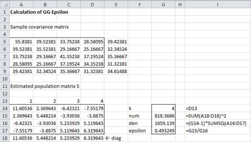
Example 1: Calculate the value of the GG epsilon for Example 1 of ANOVA with Repeated Measures with One Within Subjects Factor using the above approach.
Figure 1 – Calculation of GG epsilon for Example 1
Range A5:D8 in Figure 1 contains the sample covariance matrix (see Figure 3 of Sphericity). E5:E8 contains the row means and A9:D9 contains the column means. E9 contains the grand mean.
Range A14:D17 contains the estimated population matrix as described above. E.g. cell A15 contains the formula =A6-$E6-A$9+$E$9. The elements in row 18 are the values of the diagonal of this matrix formed in the usual way (e.g. cell B18 contains the formula =INDEX(B14:B17,B13).
The value of the GG epsilon is 0.493 (cell F17) is the same as that calculated previously (see Figure 3 of Sphericity).
Approach using Eigenvalues
An alternative way of calculating GG epsilon is using the k-1 non-zero eigenvalues λj of matrix S, as follows:
See Example 1 of Goal Seeking and Solver for the definition of an eigenvalue and a way of calculating it. The Real Statistics function eVALUES can also be used to calculate the eigenvalues of a matrix as described in Eigenvalues and Eigenvectors.
Example 2: Calculate the value of the GG epsilon for Example 1 using the eigenvalues of matrix .
Figure 2 – Calculation of GG epsilon for using eigenvalues
The results are given in Figure 2. The eigenvalues of matrix S are produced by highlighting cells A22:C22 (k–1 = 3 cells) and entering the Real Statistics array formula =eVALUES(A14:D17). The value of GG epsilon (cell G25) is once again .493.
Mauchly’s test for sphericity
We now present Mauchly’s test, a commonly used test to determine whether the sphericity assumption holds. Because of its lack of power, Mauchly’s test is not recommended and in fact, it is simply better to apply either the GG or HF epsilon correction factor in all cases. We also present John, Nagao and Sugiura’s test for sphericity, a much more powerful and useful test.
Property 1: (Mauchly’s test) Define the following statistics based on the k-1 non-zero eigenvalues of the matrix S described above:

![]()
If W = 1 then the original data meets the sphericity assumption. If the original data meets the sphericity assumption (the null hypothesis) then
![]()
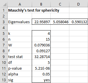
Example 3: Determine whether the data in Example 1 meets Mauchly’s test for sphericity.
Figure 3 – Mauchly’s test for sphericity
From Figure 3, we reject the null hypothesis and conclude that the sphericity assumption has not been met.
John, Nagao and Sugiura’s test
Property 2: (John, Nagao and Sugiura’s test): Define the following statistics based on the k-1 non-zero eigenvalues of the matrix S described above:
If the original data meets the sphericity assumption (the null hypothesis) then
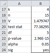
Example 4: Determine whether the data in Example 1 meets the John, Nagao and Sugiura test for sphericity.
Figure 4 – John, Nagao and Sugiura’s test for sphericity
This test even more definitively shows (see Figure 4) that the data does not meet the sphericity assumption.
Real Statistics Tests for Sphericity
Real Statistics Functions: The following functions implement the two tests for sphericity described above on the data in range R1 in Excel format for one-way repeated measures ANOVA.
MauchlyTest(R1) = p-value of Mauchly’s test for sphericity on the data in range R1
JNSTest(R1) = p-value of the John-Nagao-Sugiura test for sphericity on the data in R1
Note that for Example 1 (based on the data in Figure 1), MauchlyTest(H6:K20) = 5.21E-06 and JNSTest(H6:K20) = 2.96E-15 (consistent with the results shown in Figures 3 and 4).
Examples Workbook
Click here to download the Excel workbook with the examples described on this webpage
References
Nimon, K., Williams, V. (2020) Evaluating performance improvement through repeated measures: a primer for educators considering univariate and multivariate designs
https://imaging.mrc-cbu.cam.ac.uk/statswiki/FAQ/Mauchly?action=AttachFile&do=view&target=sphericity.pdf
Watson, P. (2023) What is the formula for Mauchly’s W used for testing sphericity in univariate repeated measures anova?
https://imaging.mrc-cbu.cam.ac.uk/statswiki/FAQ/Mauchly
Maxwell S. E., Delaney H. D. (2004). Designing experiments and analyzing data: a model comparison perspective, 2nd edn. Mahwah, NJ: Erlbaum
https://api.pageplace.de/preview/DT0400.9781135653477_A23806531/preview-9781135653477_A23806531.pdf


Dear Sir,
I have 3 independent samples and one of eigenvalues is zero. How can I use Mauchly’s Test because the natural logarithm of zero is undefined?
Nat,
If the three samples are truly independent then the covariance matrix would be a diagonal matrix with the variances on the diagonal and zeros everywhere else. The variances would then be the eigenvalues, This would mean that the variance of one of the samples would be zero, i.e. all the elements in this sample are equal. Is this really your situation?
In any case a zero eigenvalue would mean that the covariance matrix is not invertible and so all the usual approaches would not work. In particular Mauchly’s test wouldn’t work.
If you send me an Excel file with your data I can try to figure out what is going on.
Charles
Charles
Sir,
I am so sorry! I have 3 dependent samples. My S-matrix as follows:
2.555 −1.695 −0.859
−1.695 2.441 −0.746
−0.859 −0.746 1.605
I used Excel (or Mathematica or Maple or Matlab) to find eigenvalues of S and had 3 eigenvalues: λ_1 = 4.199, λ_2 = 2.402 và λ_3 = 0. If I use the product λ_1. λ_2. λ_3 , I get W=0. I remove the zero eigenvalue then the W statistic becomes normally! SPSS also gives the result like that. So, can we remove the zero eigenvalues in general?
Nat,
This is a very strange S matrix. Note that if you invert the S matrix you get a matrix all of whose elements are 1000.
It would be good to see the original data from which the S matrix was generated to see why you are getting this result.
Charles
Thanks Sir!