Within-subjects assumptions| Real Statistics Using Excel

Basic Concepts

The assumptions that need to be met for the repeated measures analysis described in Example 1 of One Between-Subjects Factor and One Within-Subjects Factor to be valid fall into two categories: assumptions for the between-subjects analysis and those for the within-subjects analysis. We will focus on the within-subjects analysis on this webpage.

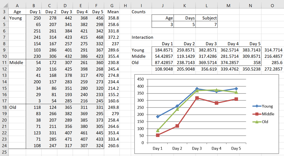
The data for Example 1 is repeated on the left side of Figure 1.

Figure 1 – Data for Example 1

Assumptions

For the within-subjects tests to be valid the following assumptions need to be satisfied:

All samples are drawn from normally distributed populations
The Days × Subjects population covariance matrices at each Age level are approximately equal, which in Example 1 means that Σ_Young ≈ Σ_Middle ≈ Σ_Old
Σ satisfies the sphericity assumption

Normality

We need to test each of the 15 Days × Age samples for normality (or at least symmetry). From the box plot, we see in Figure 2 that this assumption is reasonably well satisfied.

Figure 2 – Box plots of Days × Age samples

Equality of Covariance Matrices

Since we don’t have access to the population covariance matrices, we test the equality of the sample covariance matrices. Box’s M test can be used for this combined with Levene’s test for homogeneity of variances. Figure 3 shows the result of Levene’s test for Day 1.

Figure 3 – Levene’s test for Day 1 within-subjects factor

We can see that the variances are 5118, 4378, and 938, but the p-value of .09 > .05 shows that the variances are equal enough for our purposes. Levene’s test on the other days shows that they too satisfy the homogeneity of variance assumption.

Box’s test for equality of covariance matrices yields the following result: M = 34.81, (30, 1027) = .67, p-value = .91 > .05 = α, and so we can conclude there are no significant differences between the covariance matrices. Click here for the details about how to use Box’s Test for the Equivalence of Covariance Matrices.

Sphericity

As usual, instead of checking for sphericity, we will simply adjust the degrees of freedom to compensate for the lack of sphericity by using Greenhouse and Geisser’s epsilon:

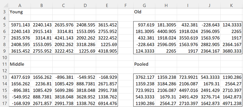
where k = the number of days (k = 5 in our example) and S is the sample covariance matrix. Since we are assuming that Σ_Young ≈ Σ_Middle ≈ Σ_Old, it is sufficient to use the pooled sample covariance matrix (i.e. the average of the three group-level covariance matrices). In our example, the three sample covariance matrices and the pooled matrix are shown in Figure 4.

Figure 4 – Covariance matrices for Example 1

The value of $\hat\epsilon_{GG}$ is calculated from the pooled covariance matrix exactly as was done in Figure 3 of Sphericity. See Figure 5.

Figure 5 – Calculation of GG epsilon and HF epsilon

The HF epsilon is calculated by the formula used in Sphericity, namely

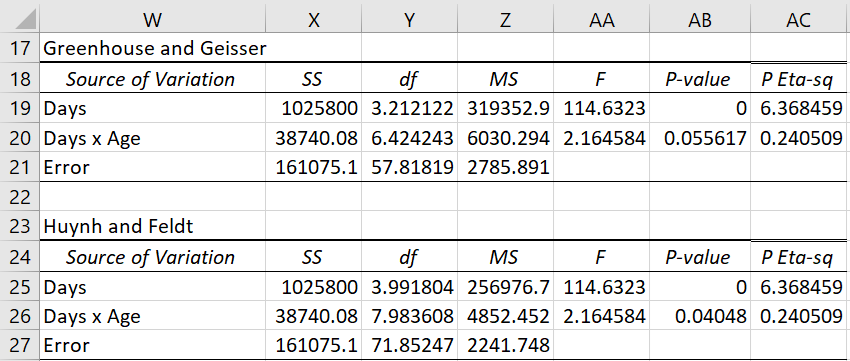
Here k = # of days = 5 and n = # subjects ∙ # Age groups = 7 ∙ 3 = 21. Thus, GG epsilon = .80 (cell BB44) and HF epsilon = .998 (cell BB47). Since GG epsilon > .75, we should use the HF epsilon correction factor. Since this is almost 1, it is safe to assume sphericity. In any case, the revised version of the omnibus ANOVA test from Figure 4 of One Between-Subjects Factor and One Within-Subjects Factor for the within-subjects factor is shown in Figure 6.

Figure 6 – Within-subjects ANOVA corrected for sphericity

Examples Workbook

Click here to download the Excel workbook with the examples described on this webpage.

Reference

Howell, D. C. (2010) Statistical methods for psychology (7^th ed.). Wadsworth, Cengage Learning.
https://labs.la.utexas.edu/gilden/files/2016/05/Statistics-Text.pdf

Assumptions for within-subjects analysis