Detailed Between-Subjects Analysis

Basic Concepts

On this webpage, we provide a more detailed analysis of the between-subjects factor for Example 1 of One Between-Subjects Factor and One Within-Subjects Factor.

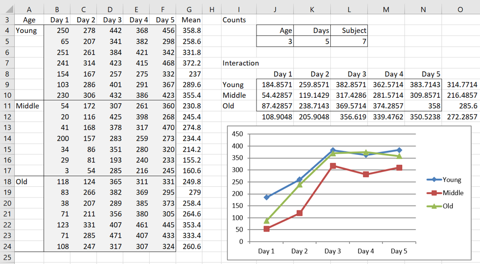
The data for Example 1 is repeated on the left side of Figure 1.

Figure 1 – Data for Example 1

Ignoring Time Intervals

We know from cell U8 of Figure 4 of One Between-Subjects Factor and One Within-Subjects Factor that there is a significant difference between the different Age groups. p-value = .002789. If we want to investigate these differences further, we can perform a one-way ANOVA on the data in column G of Figure 1.

Using the array formula =RESHAPE(G4:G24) in range I4:K10 of Figure 2, we reformat the data in column G for one-way ANOVA. The p-value for this ANOVA, using the formula =ATEST(I4:K10), is .002789, which matches the value referenced above. 

Figure 2 – Between-subjects comparisons

What we are interested in, however, are the pairwise comparisons, which we can obtain by using Tukey’s HSD, as shown on the right side of Figure 2. We see that Young-Middle and Middle-Old are significant, but Young-Old are not.

Simple Effects based on Time Intervals

For the between-subjects simple effects since we only use one Days level at a time, we don’t need to worry about sphericity, and as a result, we can and should use a pooled error term.

Let’s begin by looking at the simple effects of Age vs. Day 1 and Age vs. Day 5. Essentially we compute one-way ANOVA with independent variables but with a pooled error term (see Figure 3).

Figure 3 – ANOVA for Age × Day 1 and Age × Day 5

Simple effects ANOVA

As we did to build the table in Figure 4 of One Between-Subjects Factor and One Within-Subjects Factor, we can build the two simple effects ANOVAs from the table in the top part of Figure 3. Figure 4 displays key formulas for the Age × Day 1 analysis in that table (referring to cells in Figure 1). The formulas for Age × Day 5 are similar.

Now

is the pooled error term and is used for both the Age × Day 1 and Age × Day 5 analyses. Unfortunately, the value calculated for F in Figure 3 is not really distributed as F(2, 90) as indicated. The problem is that the error term is the sum of two possibly heterogeneous sources of error. To address this we need to recalculate df in the same manner as we did in Property 1 of Two Sample t Test with Unequal Variances.

Using subscript 1 for the first error term (Subj w/i Age) and subscript 2 for the second error term (Days × Subj w/i Age), we calculate the following revised value of df.

Figure 5 shows the revised version of Figure 3.

Figure 5 – Corrected ANOVA for Age × Day 1 and Age × Day 5

This tells us there is a significant difference between the three Age groups on Day 1, but no significant difference on Day 5.

Examples Workbook

Click here to download the Excel workbook with the examples described on this webpage.

Reference

Howell, D. C. (2010) Statistical methods for psychology (7^th ed.). Wadsworth, Cengage Learning.
https://labs.la.utexas.edu/gilden/files/2016/05/Statistics-Text.pdf