Basic Concepts
The one random factor structural model is given by the formula
As usual, εij can be considered to be random variables with variance , but unlike in the fixed factor case, this time τj can be considered to be a random variable (instead of a constant) with variance
.
We assume that for all i and j, and
are pairwise independent and
Since and
are independent it follows that
We test the null and alternative hypotheses
H0: = 0 H1;
≥ 0
Note that the null hypothesis is equivalent to ≤ 0. If the null hypothesis is true, then variability among the randomly selected treatments is simply due to random error (i.e.
). If the alternative hypothesis is true then variability among the randomly selected treatments is significantly higher than just the random error.
The definitions of SST, SSB, SSE, and similarly for the MS and df terms, are exactly the same as for the one fixed factor model described in One-way Anova Basic Concepts. In fact, the calculations are also the same, although the interpretation of the results is different.
Using the notation for one-way ANOVA with fixed effects
![]()
where
![]()
For a balanced model m = n/k. If the null hypothesis is true, then = 0, and so
If the alternative hypothesis is true, then ≠ 0, and so
Estimates of Variances
We first note that we can estimate by MSE and
by
(provided MSB > MSE). With a balanced model, we can construct a confidence interval for based on
Assuming a balanced model, we can construct (Satterthwaite) a confidence interval for based on
As usual, the population mean can be estimated by the grand mean, μ = E[x̄]. The variance of this estimate is (m +
)/(km), which can be estimated by MSA/(km).
Data Analysis
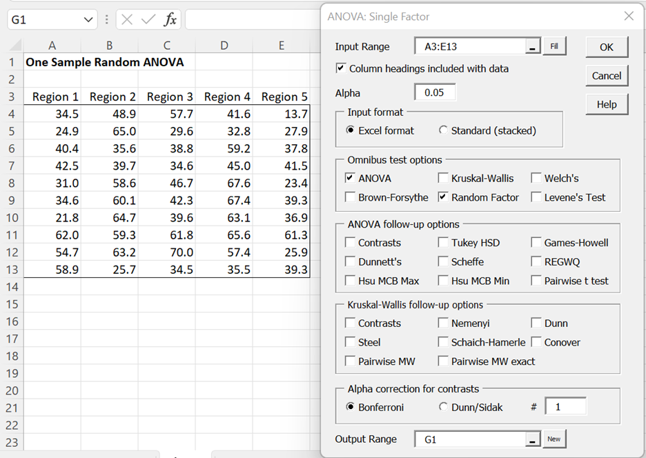
Example 1: A biologist is trying to determine whether the toxicity of a certain type of mushroom is the same across the 100 different regions being studied. She takes a random sample of 5 of these regions and then measures the toxicity of 10 mushrooms selected at random in each of the selected regions. Determine whether there is a significant difference in the toxicity of these mushrooms in different regions based on the data on the left side of Figure 1.
Figure 1 – One Random Factor Anova dialog box
To run the analysis you can use Excel’s Anova: Single Factor data analysis tool, as described in One-way Anova Basic Concepts. Alternatively, you can use the Real Statistics One Factor Factor Anova data analysis tool, as follows, since it provides some additional information.
For Example 1, enter Ctrl-m and select Anova: one factor from the Anova tab. (If using the original user interface, double click on the Analysis of Variance option and select Anova: one factor from the dialog box that appears). Fill in the dialog box that now appears as shown on the right side of Figure 1. This is the same procedure that is used for one fixed factor Anova, except that you now check the Random Factor option.
Results
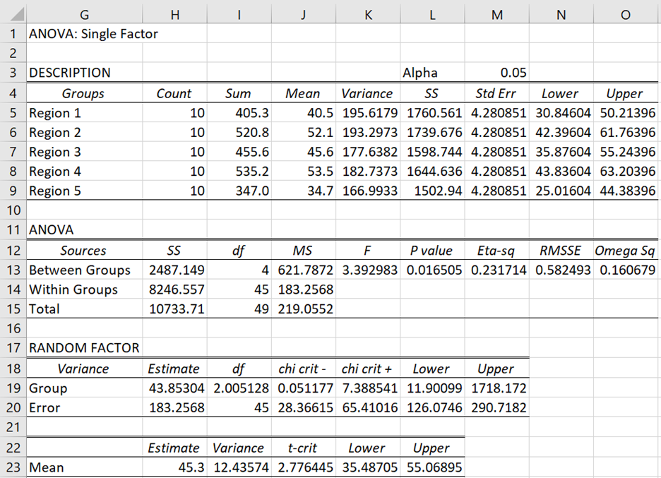
Figure 2 displays the output.
Figure 2 – One Random Factor ANOVA data analysis
The first part of the analysis is identical to the output when the Random Factor option is not checked. As we can see from Figure 2 cell L13, p-value = .0165. Assuming that α = .05, we conclude there is a significant difference in the toxicity of the mushroom under study among the 100 regions.
The second part of the output provides an estimate of the mean toxicity of the mushroom across the 100 regions (cell H23) and a 95% confidence interval (cells K23 and L23), as well as estimates of the population between groups variance and error variance (cells H19 and H20) and their 95% confidence intervals (cells L19, L20, and M19, M20).
Cautions
As mentioned previously, the above estimates assume that MSB > MSE. When this is not the case, a negative variance will occur, which is of course impossible, and so the estimates should be ignored. Also, if the degrees of freedom for the between-groups variance (cell I19) is low then the confidence interval will be large, and so will not be very useful. In fact, if the value of df is less than one, Excel will round it down to zero when calculating the chi-square values (cells J19 and K19) resulting in an error. For this reason, the data analysis tool uses the Real Statistics function CHISQ_INV instead of CHISQ.INV.
Examples Workbook
Click here to download the Excel workbook with the examples described on this webpage.
References
Howell, D. C. (2010) Statistical methods for psychology (7th ed.). Wadsworth, Cengage Learning.
https://labs.la.utexas.edu/gilden/files/2016/05/Statistics-Text.pdf
PennState (2023) Random effects and introduction to mixed models
https://online.stat.psu.edu/stat502/lesson/6


Dear professor,
How to run one random factor nested ANOVA in R software?
Thanks you.
Sorry, but I don’t use R.
Charles
Charles,
In your example above, your software calculates cell I23 by H19/(nk)– it should have been MSB/(nk), or cell J13/(nk) = 12.44.
Heather,
You are correct. I have just corrected the referenced webpage. I will correct the examples workbook when I release a new version in a few days. Thanks for catching this mistake.
Charles
I do not think this was corrected, as I still see the formula H19/nk.
Hello Edita,
Thanks for bringing this to my attention. I thought that I had corrected this a long time ago. I have now highlighted this problem on the webpage and will correct it in the next bug-fix release of the Real Statistics software, Rel 8.3.2 (I have just made the correction in the code).
I really appreciate your diligence and your assistance in improving the quality of the Real Statistics software.
Charles